Sample Solution

BPHCT-135 Solved Assignment

PART A
  1. a) Discuss Regnault’s experiments on Hydrogen, nitrogen and carbon dioxide for 273 K. Also discuss the Andrews experiments for CO 2 CO 2 CO_(2)\mathrm{CO}_2CO2 on the p V p V p-Vp-VpV diagram at various temperatures.
    b) Write the assumptions made by Maxwell to derive the expression for distribution function of velocities. Hence derive the expression of Maxwellian distribution function for molecular speeds. Plot Maxwellian distribution function as a function of molecular speed.
    c) The average speed of hydrogen molecules is 1850 ms 1 1850 ms 1 1850ms^(-1)1850 \mathrm{~ms}^{-1}1850 ms1. The radius of a hydrogen molecule is 1.40 × 10 10 m 1.40 × 10 10 m 1.40 xx10^(-10)m1.40 \times 10^{-10} \mathrm{~m}1.40×10¹⁰ m. Calculate (i) Collision cross-section, (ii) collision frequency, and (iii) mean free path. Take n = 3 × 10 25 m 3 n = 3 × 10 25 m 3 n=3xx10^(25)m^(-3)n=3 \times 10^{25} \mathrm{~m}^{-3}n=3×1025 m3.
    d) What is Brownian motion? Discuss Perrin’s method for determination of Avogadro number in Brownian motion. How can this method be used to estimate the mass of molecule
  2. a) Explain the classification of boundaries in a thermodynamic system.
    b) State Zeroth law of thermodynamics. How does this law introduces the concept of temperature. Write parametric as well as exact equation of state for one mole of a ideal gas and stretched wire.
    c) Show that for an ideal gas
α = 1 T and β T = 1 p α = 1 T and β T = 1 p alpha=(1)/(T)” and “beta _(T)=(1)/(p)\alpha=\frac{1}{T} \text { and } \beta_T=\frac{1}{p}α=1T and βT=1p
where β T β T beta _(T)\beta_TβT is the isothermal compressibility and α α alpha\alphaα is isobaric coefficient of volume expansion.
d) Derive Mayer’s formula: C p C V = R C p C V = R C_(p)-C_(V)=RC_p-C_V=RCpCV=R where C p C p C_(p)C_pCp and C V C V C_(V)C_VCV are the molar heat capacity at constant pressure and constant volume respectively.
e) Obtain an expression for work done in expanding a gas from volume V i V i V_(i)V_iVi to V f V f V_(f)V_fVf in an isobaric process.
PART B
3. a) With the help of entropy – temperature diagram of Carnot cycle, obtain an expression of efficiency of a Carnot engine. A Carnot engine has an efficiency of 50 % 50 % 50%50 \%50%. It operates between reservoirs of constant temperature with temperature difference of 80 K . Calculate the temperature of the low-temperature reservoir in Celsius.
b) Define thermodynamic potentials. Derive Maxwell’s relations from thermodynamic potentials.
c) When two phases of a substance coexist in equilibrium at constant temperature and pressure, their specific Gibb’s free energies are equal. Using this fact, obtain Clausius-Clapeyron equation.
d) Derive Planck’s law of radiation and hence obtain Rayleigh-Jeans law and Wien’s law.
4. a) Consider a classical ideal gas consisting of N N NNN particles. The energy ε ε epsi\varepsilonε of a particle is given by ε = c p ε = c p epsi=cp\varepsilon=c pε=cp where c c ccc is a constant and p p ppp is the magnitude of the momentum. Calculate (i) the partition function of the system, (ii) internal energy, and (iii) C V C V C_(V)C_VCV.
b) 5.4 × 10 21 5.4 × 10 21 5.4 xx10^(21)5.4 \times 10^{21}5.4×10²¹ electrons are confined in a box of volume 1 cm 3 1 cm 3 1cm^(3)1 \mathrm{~cm}^31 cm3. Calculate their Fermi wavelength and Fermi energy.
c) Define thermodynamic probability of a macrostate. Establish the Boltzmann relation between entropy and thermodynamic probability:
S = k B ln W S = k B ln W S=k_(B)ln WS=k_{\mathrm{B}} \ln WS=kBlnW
d) Obtain an expression of Fermi-Dirac distribution function. Plot Fermi function versus energy at different temperatures.

Answer:

Question:-1

a) Discuss Regnault’s experiments on Hydrogen, Nitrogen, and Carbon Dioxide for 273 K. Also, discuss Andrews’ experiments for CO 2 CO 2 CO_(2)\mathrm{CO}_2CO2 on the p V p V p-Vp-VpV diagram at various temperatures.

Answer:

Regnault’s Experiments on Hydrogen, Nitrogen, and Carbon Dioxide at 273 K

Henri Victor Regnault conducted extensive experiments in the 19th century to study the behavior of gases, particularly focusing on deviations from the ideal gas law, P V = n R T P V = n R T PV=nRTPV = nRTPV=nRT, at various temperatures and pressures. His work on hydrogen ( H 2 H 2 H_(2)H_2H2), nitrogen ( N 2 N 2 N_(2)N_2N2), and carbon dioxide ( C O 2 C O 2 CO_(2)CO_2CO2) at 273 K (0°C, the ice point) provides valuable insights into the real gas behavior of these substances.

1. Context and Methodology

Regnault’s experiments were aimed at understanding how real gases deviate from ideal behavior, particularly under conditions of high pressure and low temperature. At 273 K, which is close to standard conditions, gases are expected to exhibit noticeable deviations due to intermolecular forces and molecular volume effects. Regnault used precise measurement techniques to determine the compressibility factor Z = P V n R T Z = P V n R T Z=(PV)/(nRT)Z = \frac{PV}{nRT}Z=PVnRT, which quantifies the departure from ideality ( Z = 1 Z = 1 Z=1Z = 1Z=1 for an ideal gas).

2. Observations at 273 K

  • Hydrogen ( H 2 H 2 H_(2)H_2H2):
    Hydrogen, being a small and non-polar molecule with weak intermolecular forces, exhibits behavior closer to an ideal gas than most other gases. At 273 K, Regnault observed that the P V P V PVPVPV product for hydrogen increases with increasing pressure, indicating a Z > 1 Z > 1 Z > 1Z > 1Z>1. This positive deviation arises because the molecular volume of hydrogen is negligible, and repulsive forces dominate at higher pressures. The curve of P V P V PVPVPV versus P P PPP (Amagat’s curve) for hydrogen shows a steady rise, reflecting its resistance to compression.
  • Nitrogen ( N 2 N 2 N_(2)N_2N2):
    Nitrogen, a diatomic and non-polar molecule, shows moderate deviations from ideal behavior at 273 K. Regnault found that the P V P V PVPVPV product initially decreases with increasing pressure, reaching a minimum, and then rises at higher pressures. This behavior indicates Z < 1 Z < 1 Z < 1Z < 1Z<1 at low pressures due to attractive intermolecular forces and Z > 1 Z > 1 Z > 1Z > 1Z>1 at high pressures due to the dominance of molecular volume effects. The minimum in the P V P V PVPVPV curve reflects the balance between these competing effects.
  • Carbon Dioxide ( C O 2 C O 2 CO_(2)CO_2CO2):
    Carbon dioxide, with its larger molecular size and stronger intermolecular forces (due to its quadrupole moment), exhibits significant deviations from ideal behavior at 273 K. Regnault observed that the P V P V PVPVPV product decreases sharply with increasing pressure, indicating Z < 1 Z < 1 Z < 1Z < 1Z<1, before rising at very high pressures. This pronounced negative deviation is attributed to the strong attractive forces between C O 2 C O 2 CO_(2)CO_2CO2 molecules, which are particularly significant near 273 K, a temperature close to the critical temperature of C O 2 C O 2 CO_(2)CO_2CO2 (304.1 K). The P V P V PVPVPV curve for C O 2 C O 2 CO_(2)CO_2CO2 passes through a deep minimum, highlighting its tendency to be easily liquefied.

3. Key Conclusions from Regnault’s Work

  • Regnault’s experiments demonstrated that the behavior of real gases depends on their molecular properties, such as size, polarity, and intermolecular forces. At 273 K:
    • Gases like hydrogen, with weak attractive forces, show positive deviations ( Z > 1 Z > 1 Z > 1Z > 1Z>1) and resist compression.
    • Gases like nitrogen, with moderate intermolecular forces, exhibit a balance between attractive and repulsive effects, leading to a minimum in the P V P V PVPVPV curve.
    • Gases like carbon dioxide, which are easily liquefied, show strong negative deviations ( Z < 1 Z < 1 Z < 1Z < 1Z<1) due to dominant attractive forces.
  • These findings challenged the ideal gas law and laid the groundwork for the development of more accurate equations of state, such as the van der Waals equation, which account for molecular interactions and finite molecular volumes.

Andrews’ Experiments on Carbon Dioxide and the p V p V p-Vp-VpV Diagram at Various Temperatures

Thomas Andrews conducted pioneering experiments on carbon dioxide ( C O 2 C O 2 CO_(2)CO_2CO2) in the 1860s, focusing on its behavior under varying pressures and temperatures. His work led to the discovery of the critical point and the development of the p V p V p-Vp-VpV diagram, which is a fundamental tool in understanding phase transitions and real gas behavior. Below, I discuss Andrews’ experiments and the key features of the p V p V p-Vp-VpV isotherms for C O 2 C O 2 CO_(2)CO_2CO2:

1. Experimental Setup

Andrews used a high-pressure apparatus consisting of strong capillary tubes and a screw mechanism to compress C O 2 C O 2 CO_(2)CO_2CO2. Nitrogen was used as a reference gas to estimate pressure, assuming it obeyed Boyle’s law under the experimental conditions. He plotted a series of p V p V p-Vp-VpV isotherms (constant-temperature curves) to study the behavior of C O 2 C O 2 CO_(2)CO_2CO2 over a wide range of pressures and temperatures.

2. Key Features of the p V p V p-Vp-VpV Diagram

Andrews’ experiments revealed distinct behaviors of C O 2 C O 2 CO_(2)CO_2CO2 at different temperatures, which are summarized below:
original image
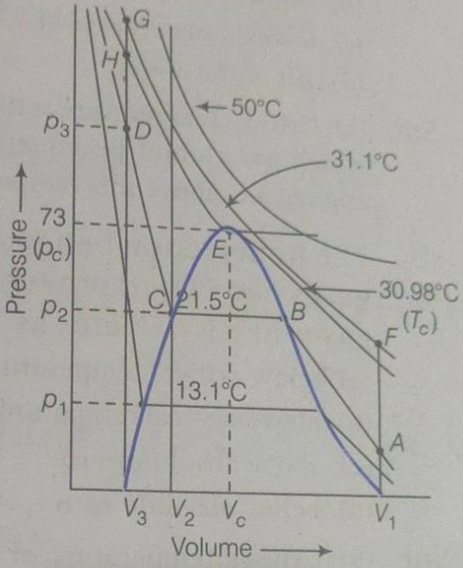
  • Above the Critical Temperature ( T > 30.9 C T > 30.9 C T > 30.9^(@)”C”T > 30.9^\circ \text{C}T>30.9C):
    • At temperatures above 30.9°C (the critical temperature of C O 2 C O 2 CO_(2)CO_2CO2), Andrews observed that C O 2 C O 2 CO_(2)CO_2CO2 behaves as a supercritical fluid and cannot be liquefied by pressure alone. The p V p V p-Vp-VpV isotherms are smooth and continuous, resembling the hyperbolic curves of an ideal gas but with deviations due to real gas effects. For example, at 50°C, the isotherm closely follows Boyle’s law at moderate pressures but shows deviations at higher pressures due to molecular volume effects.
  • At the Critical Temperature ( T = 30.9 C T = 30.9 C T=30.9^(@)”C”T = 30.9^\circ \text{C}T=30.9C):
    • At 30.9°C, Andrews identified the critical point of C O 2 C O 2 CO_(2)CO_2CO2, where the distinction between liquid and vapor phases disappears. The p V p V p-Vp-VpV isotherm at this temperature exhibits an inflection point, marking the critical pressure ( P c = 73.8 atm P c = 73.8 atm P_(c)=73.8″atm”P_c = 73.8 \, \text{atm}Pc=73.8atm) and critical volume. The critical point is characterized by the conditions where the meniscus between liquid and vapor vanishes, and the substance exists as a single phase with unique properties.
  • Below the Critical Temperature ( T < 30.9 C T < 30.9 C T < 30.9^(@)”C”T < 30.9^\circ \text{C}T<30.9C):
    • At temperatures below 30.9°C, Andrews observed phase transitions between liquid and vapor states. The p V p V p-Vp-VpV isotherms exhibit a horizontal segment (a "tie line") corresponding to the coexistence of liquid and vapor phases at constant pressure (the vapor pressure). For example:
      • At 0°C (273 K), the isotherm shows a horizontal line where liquid and vapor C O 2 C O 2 CO_(2)CO_2CO2 coexist, and increasing pressure results in complete liquefaction.
      • As the temperature decreases further (e.g., below 0°C), the vapor pressure decreases, and the horizontal segment of the isotherm shifts to lower pressures.
    • Outside the coexistence region, the isotherms show steep slopes in the liquid phase (indicating low compressibility) and gradual slopes in the vapor phase (indicating higher compressibility).

3. Significance of Andrews’ Findings

  • Discovery of the Critical Point: Andrews’ identification of the critical temperature (30.9°C), critical pressure (73.8 atm), and critical volume for C O 2 C O 2 CO_(2)CO_2CO2 was a groundbreaking contribution to thermodynamics. The critical point marks the boundary beyond which a substance cannot exist in distinct liquid and vapor phases, transitioning instead to a supercritical fluid state.
  • Continuity of States: Andrews demonstrated the "continuity of states," showing that liquid and vapor phases are not fundamentally distinct but can transform into each other continuously under certain conditions. This concept challenged earlier views of phase transitions and influenced the development of modern theories of critical phenomena.
  • Behavior Below and Above Critical Temperature: Andrews’ p V p V p-Vp-VpV diagrams highlighted the qualitative differences in C O 2 C O 2 CO_(2)CO_2CO2 behavior above and below the critical temperature. Above T c T c T_(c)T_cTc, C O 2 C O 2 CO_(2)CO_2CO2 remains a single phase, while below T c T c T_(c)T_cTc, it undergoes phase separation, with the liquid-vapor coexistence region bounded by the dashed line (Maxwell’s construction) on the p V p V p-Vp-VpV diagram.

4. Implications for Real Gas Behavior

Andrews’ experiments underscored the limitations of the ideal gas law and provided empirical evidence for the development of equations of state that account for phase transitions and critical phenomena. His work on C O 2 C O 2 CO_(2)CO_2CO2 inspired subsequent researchers, such as van der Waals, to formulate equations that describe the behavior of real gases and liquids near and beyond the critical point.

Comparison and Broader Context

  • Regnault vs. Andrews: While Regnault focused on the deviations of gases from ideal behavior at specific temperatures (e.g., 273 K) and high pressures, Andrews explored the phase behavior of C O 2 C O 2 CO_(2)CO_2CO2 across a range of temperatures, emphasizing the critical point and phase transitions. Regnault’s work provided quantitative data on compressibility, whereas Andrews’ experiments offered qualitative insights into the continuity of states and the p V p V p-Vp-VpV relationship.
  • Critical Examination of Narratives: The established narrative often credits Andrews with the discovery of the critical point, but it is worth noting that Regnault’s earlier work on real gas deviations laid essential groundwork. Additionally, while Andrews’ experiments were groundbreaking, they relied on assumptions (e.g., nitrogen obeying Boyle’s law) that may not hold at extreme conditions, highlighting the need for critical scrutiny of historical data.
In summary, Regnault’s experiments at 273 K revealed the distinct real gas behaviors of hydrogen, nitrogen, and carbon dioxide, while Andrews’ p V p V p-Vp-VpV diagrams for C O 2 C O 2 CO_(2)CO_2CO2 elucidated the critical point and phase transitions, shaping our understanding of thermodynamics and phase equilibria.

b) Write the assumptions made by Maxwell to derive the expression for the distribution function of velocities. Hence derive the expression of Maxwellian distribution function for molecular speeds. Plot Maxwellian distribution function as a function of molecular speed.

Answer:

To address the query, we will first outline the assumptions made by James Clerk Maxwell to derive the distribution function of velocities, then derive the Maxwellian distribution function for molecular speeds, and finally discuss how to plot the distribution as a function of molecular speed.

1. Assumptions Made by Maxwell

Maxwell developed his velocity distribution function for an ideal gas by making the following key assumptions:
  1. Ideal Gas Behavior: The gas consists of a large number of non-interacting particles (molecules) that obey the ideal gas law, P V = n R T P V = n R T PV=nRTPV = nRTPV=nRT. This implies that intermolecular forces are negligible, and the particles only interact through elastic collisions.
  2. Random Motion: The motion of the particles is completely random, and their velocities are distributed isotropically in three-dimensional space. There is no preferred direction for the velocity vectors.
  3. Statistical Equilibrium: The system is in thermal equilibrium, meaning the distribution of velocities does not change with time. The gas is at a constant temperature T T TTT, and the particles follow the laws of classical statistical mechanics.
  4. Independence of Velocity Components: The velocity of a particle in three-dimensional space can be decomposed into three mutually perpendicular components ( v x , v y , v z v x , v y , v z v_(x),v_(y),v_(z)v_x, v_y, v_zvx,vy,vz), and these components are statistically independent. This means the probability distribution for each component can be treated separately.
  5. Maxwell-Boltzmann Statistics: The particles obey classical Maxwell-Boltzmann statistics, implying that they are distinguishable and there are no quantum effects (valid for dilute gases at high temperatures).
  6. Equipartition of Energy: The kinetic energy of the particles is distributed equally among the three degrees of freedom, consistent with the equipartition theorem. The average kinetic energy per particle is 3 2 k T 3 2 k T (3)/(2)kT\frac{3}{2} kT32kT, where k k kkk is the Boltzmann constant and T T TTT is the absolute temperature.
  7. Gaussian Distribution for Velocity Components: Maxwell assumed that the distribution of each velocity component ( v x , v y , v z v x , v y , v z v_(x),v_(y),v_(z)v_x, v_y, v_zvx,vy,vz) follows a Gaussian (normal) distribution, centered at zero, due to the random nature of the motion and the central limit theorem.
These assumptions allowed Maxwell to derive a mathematical expression for the distribution of velocities, which he later extended to the distribution of speeds.

2. Derivation of the Maxwellian Distribution Function for Molecular Speeds

The Maxwellian distribution function describes the probability density of finding a molecule with a speed v v vvv in the range v v vvv to v + d v v + d v v+dvv + dvv+dv. Let’s derive this step by step.

Step 1: Velocity Distribution Function

Maxwell started by considering the velocity components v x , v y , v z v x , v y , v z v_(x),v_(y),v_(z)v_x, v_y, v_zvx,vy,vz in three-dimensional space. Based on the assumptions of isotropy and independence, the probability density for each component follows a Gaussian distribution. The probability density for v x v x v_(x)v_xvx is:
f ( v x ) = ( m 2 π k T ) 1 / 2 exp ( m v x 2 2 k T ) , f ( v x ) = m 2 π k T 1 / 2 exp m v x 2 2 k T , f(v_(x))=((m)/(2pi kT))^(1//2)exp(-(mv_(x)^(2))/(2kT)),f(v_x) = \left( \frac{m}{2\pi kT} \right)^{1/2} \exp\left( -\frac{m v_x^2}{2kT} \right),f(vx)=(m2πkT)1/2exp(mvx22kT),
where m m mmm is the mass of a molecule, k k kkk is the Boltzmann constant, and T T TTT is the temperature. Similar expressions apply to v y v y v_(y)v_yvy and v z v z v_(z)v_zvz.
Since the components are independent, the joint probability density for the velocity vector v = ( v x , v y , v z ) v = ( v x , v y , v z ) v=(v_(x),v_(y),v_(z))\mathbf{v} = (v_x, v_y, v_z)v=(vx,vy,vz) is the product of the individual distributions:
f ( v x , v y , v z ) = f ( v x ) f ( v y ) f ( v z ) = ( m 2 π k T ) 3 / 2 exp ( m ( v x 2 + v y 2 + v z 2 ) 2 k T ) . f ( v x , v y , v z ) = f ( v x ) f ( v y ) f ( v z ) = m 2 π k T 3 / 2 exp m ( v x 2 + v y 2 + v z 2 ) 2 k T . f(v_(x),v_(y),v_(z))=f(v_(x))*f(v_(y))*f(v_(z))=((m)/(2pi kT))^(3//2)exp(-(m(v_(x)^(2)+v_(y)^(2)+v_(z)^(2)))/(2kT)).f(v_x, v_y, v_z) = f(v_x) \cdot f(v_y) \cdot f(v_z) = \left( \frac{m}{2\pi kT} \right)^{3/2} \exp\left( -\frac{m (v_x^2 + v_y^2 + v_z^2)}{2kT} \right).f(vx,vy,vz)=f(vx)f(vy)f(vz)=(m2πkT)3/2exp(m(vx2+vy2+vz2)2kT).
The term v x 2 + v y 2 + v z 2 = v 2 v x 2 + v y 2 + v z 2 = v 2 v_(x)^(2)+v_(y)^(2)+v_(z)^(2)=v^(2)v_x^2 + v_y^2 + v_z^2 = v^2vx2+vy2+vz2=v2, where v v vvv is the speed, so:
f ( v x , v y , v z ) = ( m 2 π k T ) 3 / 2 exp ( m v 2 2 k T ) . f ( v x , v y , v z ) = m 2 π k T 3 / 2 exp m v 2 2 k T . f(v_(x),v_(y),v_(z))=((m)/(2pi kT))^(3//2)exp(-(mv^(2))/(2kT)).f(v_x, v_y, v_z) = \left( \frac{m}{2\pi kT} \right)^{3/2} \exp\left( -\frac{m v^2}{2kT} \right).f(vx,vy,vz)=(m2πkT)3/2exp(mv22kT).
This is the Maxwellian velocity distribution function in terms of the velocity vector.

Step 2: Transformation to Speed Distribution

To find the distribution of speeds, we need to convert the velocity distribution into a speed distribution. Speed v v vvv is the magnitude of the velocity vector, v = v x 2 + v y 2 + v z 2 v = v x 2 + v y 2 + v z 2 v=sqrt(v_(x)^(2)+v_(y)^(2)+v_(z)^(2))v = \sqrt{v_x^2 + v_y^2 + v_z^2}v=vx2+vy2+vz2, and we must account for the fact that many velocity vectors can correspond to the same speed.
The probability of finding a molecule with a velocity vector in the infinitesimal volume element d v x d v y d v z d v x d v y d v z dv_(x)dv_(y)dv_(z)dv_x \, dv_y \, dv_zdvxdvydvz is:
f ( v x , v y , v z ) d v x d v y d v z . f ( v x , v y , v z ) d v x d v y d v z . f(v_(x),v_(y),v_(z))dv_(x)dv_(y)dv_(z).f(v_x, v_y, v_z) \, dv_x \, dv_y \, dv_z.f(vx,vy,vz)dvxdvydvz.
To express this in terms of speed, we switch to spherical coordinates, where:
  • v x = v sin θ cos ϕ v x = v sin θ cos ϕ v_(x)=v sin theta cos phiv_x = v \sin\theta \cos\phivx=vsinθcosϕ,
  • v y = v sin θ sin ϕ v y = v sin θ sin ϕ v_(y)=v sin theta sin phiv_y = v \sin\theta \sin\phivy=vsinθsinϕ,
  • v z = v cos θ v z = v cos θ v_(z)=v cos thetav_z = v \cos\thetavz=vcosθ,
    and the volume element in spherical coordinates is:
d v x d v y d v z = v 2 sin θ d v d θ d ϕ . d v x d v y d v z = v 2 sin θ d v d θ d ϕ . dv_(x)dv_(y)dv_(z)=v^(2)sin thetadvd thetad phi.dv_x \, dv_y \, dv_z = v^2 \sin\theta \, dv \, d\theta \, d\phi.dvxdvydvz=v2sinθdvdθdϕ.
The speed distribution function f ( v ) f ( v ) f(v)f(v)f(v) is obtained by integrating over the angular variables θ θ theta\thetaθ and ϕ ϕ phi\phiϕ, which represent all possible directions for a given speed v v vvv:
f ( v ) d v = 0 π 0 2 π f ( v x , v y , v z ) v 2 sin θ d θ d ϕ d v . f ( v ) d v = 0 π 0 2 π f ( v x , v y , v z ) v 2 sin θ d θ d ϕ d v . f(v)dv=int_(0)^(pi)int_(0)^(2pi)f(v_(x),v_(y),v_(z))v^(2)sin thetad thetad phidv.f(v) \, dv = \int_0^\pi \int_0^{2\pi} f(v_x, v_y, v_z) \, v^2 \sin\theta \, d\theta \, d\phi \, dv.f(v)dv=0π02πf(vx,vy,vz)v2sinθdθdϕdv.
Substitute f ( v x , v y , v z ) f ( v x , v y , v z ) f(v_(x),v_(y),v_(z))f(v_x, v_y, v_z)f(vx,vy,vz):
f ( v ) d v = ( m 2 π k T ) 3 / 2 exp ( m v 2 2 k T ) v 2 ( 0 π sin θ d θ ) ( 0 2 π d ϕ ) d v . f ( v ) d v = m 2 π k T 3 / 2 exp m v 2 2 k T v 2 0 π sin θ d θ 0 2 π d ϕ d v . f(v)dv=((m)/(2pi kT))^(3//2)exp(-(mv^(2))/(2kT))*v^(2)*(int_(0)^(pi)sin thetad theta)(int_(0)^(2pi)d phi)dv.f(v) \, dv = \left( \frac{m}{2\pi kT} \right)^{3/2} \exp\left( -\frac{m v^2}{2kT} \right) \cdot v^2 \cdot \left( \int_0^\pi \sin\theta \, d\theta \right) \left( \int_0^{2\pi} d\phi \right) \, dv.f(v)dv=(m2πkT)3/2exp(mv22kT)v2(0πsinθdθ)(02πdϕ)dv.
Evaluate the angular integrals:
0 π sin θ d θ = [ cos θ ] 0 π = 2 , 0 2 π d ϕ = 2 π . 0 π sin θ d θ = cos θ 0 π = 2 , 0 2 π d ϕ = 2 π . int_(0)^(pi)sin thetad theta=[-cos theta]_(0)^(pi)=2,quadint_(0)^(2pi)d phi=2pi.\int_0^\pi \sin\theta \, d\theta = \left[ -\cos\theta \right]_0^\pi = 2, \quad \int_0^{2\pi} d\phi = 2\pi.0πsinθdθ=[cosθ]0π=2,02πdϕ=2π.
Thus:
f ( v ) d v = ( m 2 π k T ) 3 / 2 exp ( m v 2 2 k T ) v 2 ( 2 ) ( 2 π ) d v . f ( v ) d v = m 2 π k T 3 / 2 exp m v 2 2 k T v 2 ( 2 ) ( 2 π ) d v . f(v)dv=((m)/(2pi kT))^(3//2)exp(-(mv^(2))/(2kT))*v^(2)*(2)*(2pi)dv.f(v) \, dv = \left( \frac{m}{2\pi kT} \right)^{3/2} \exp\left( -\frac{m v^2}{2kT} \right) \cdot v^2 \cdot (2) \cdot (2\pi) \, dv.f(v)dv=(m2πkT)3/2exp(mv22kT)v2(2)(2π)dv.
Simplify:
f ( v ) d v = 4 π ( m 2 π k T ) 3 / 2 v 2 exp ( m v 2 2 k T ) d v . f ( v ) d v = 4 π m 2 π k T 3 / 2 v 2 exp m v 2 2 k T d v . f(v)dv=4pi((m)/(2pi kT))^(3//2)v^(2)exp(-(mv^(2))/(2kT))dv.f(v) \, dv = 4\pi \left( \frac{m}{2\pi kT} \right)^{3/2} v^2 \exp\left( -\frac{m v^2}{2kT} \right) \, dv.f(v)dv=4π(m2πkT)3/2v2exp(mv22kT)dv.
The Maxwellian speed distribution function f ( v ) f ( v ) f(v)f(v)f(v) is the coefficient of d v d v dvdvdv:
f ( v ) = 4 π ( m 2 π k T ) 3 / 2 v 2 exp ( m v 2 2 k T ) . f ( v ) = 4 π m 2 π k T 3 / 2 v 2 exp m v 2 2 k T . f(v)=4pi((m)/(2pi kT))^(3//2)v^(2)exp(-(mv^(2))/(2kT)).f(v) = 4\pi \left( \frac{m}{2\pi kT} \right)^{3/2} v^2 \exp\left( -\frac{m v^2}{2kT} \right).f(v)=4π(m2πkT)3/2v2exp(mv22kT).
This is the final expression for the Maxwellian distribution function for molecular speeds. It gives the probability density of finding a molecule with speed v v vvv in the range v v vvv to v + d v v + d v v+dvv + dvv+dv.

Key Features of the Distribution:

  • f ( v ) f ( v ) f(v)f(v)f(v) depends on the molecular mass m m mmm, temperature T T TTT, and speed v v vvv.
  • The factor v 2 v 2 v^(2)v^2v2 arises from the spherical volume element, reflecting the increasing number of velocity states with increasing speed.
  • The exponential term exp ( m v 2 2 k T ) exp m v 2 2 k T exp(-(mv^(2))/(2kT))\exp\left( -\frac{m v^2}{2kT} \right)exp(mv22kT) reflects the Boltzmann factor, which decreases rapidly at high speeds.

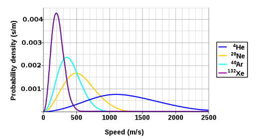
3. Plotting the Maxwellian Distribution Function

To plot f ( v ) f ( v ) f(v)f(v)f(v) as a function of molecular speed v v vvv, we need to consider its qualitative features and how it depends on m m mmm and T T TTT. The distribution has the following properties:
  1. Shape: The Maxwellian speed distribution starts at f ( 0 ) = 0 f ( 0 ) = 0 f(0)=0f(0) = 0f(0)=0, rises to a maximum at the most probable speed, and then decays exponentially at higher speeds. The curve is asymmetric and skewed toward higher speeds.
  2. Most Probable Speed ( v mp v mp v_(“mp”)v_{\text{mp}}vmp): The speed at which f ( v ) f ( v ) f(v)f(v)f(v) is maximum is found by setting the derivative d f ( v ) d v = 0 d f ( v ) d v = 0 (df(v))/(dv)=0\frac{df(v)}{dv} = 0df(v)dv=0:
    v mp = 2 k T m . v mp = 2 k T m . v_(“mp”)=sqrt((2kT)/(m)).v_{\text{mp}} = \sqrt{\frac{2kT}{m}}.vmp=2kTm.
    This is the peak of the distribution.
  3. Average Speed ( v ¯ v ¯ bar(v)\bar{v}v¯): The average speed is given by:
    v ¯ = 8 k T π m . v ¯ = 8 k T π m . bar(v)=sqrt((8kT)/(pi m)).\bar{v} = \sqrt{\frac{8kT}{\pi m}}.v¯=8kTπm.
    This lies to the right of v mp v mp v_(“mp”)v_{\text{mp}}vmp.
  4. Root-Mean-Square Speed ( v rms v rms v_(“rms”)v_{\text{rms}}vrms): The root-mean-square speed is:
    v rms = 3 k T m . v rms = 3 k T m . v_(“rms”)=sqrt((3kT)/(m)).v_{\text{rms}} = \sqrt{\frac{3kT}{m}}.vrms=3kTm.
    This is slightly higher than v ¯ v ¯ bar(v)\bar{v}v¯.
  5. Dependence on m m mmm and T T TTT:
    • For a given temperature T T TTT, lighter molecules (smaller m m mmm) have higher speeds, shifting the distribution to the right.
    • For a given mass m m mmm, higher temperatures T T TTT broaden the distribution and shift the peak to higher speeds.

Qualitative Plot Description:

  • X-Axis: Molecular speed v v vvv (in units like m/s).
  • Y-Axis: Probability density f ( v ) f ( v ) f(v)f(v)f(v) (in units like s/m).
  • Curve Shape: Starts at the origin ( v = 0 , f ( v ) = 0 v = 0 , f ( v ) = 0 v=0,f(v)=0v = 0, f(v) = 0v=0,f(v)=0), rises to a peak at v mp v mp v_(“mp”)v_{\text{mp}}vmp, and decays exponentially at large v v vvv.
  • Effect of Temperature: At higher T T TTT, the peak shifts to higher v v vvv and the curve flattens, indicating a wider range of speeds.
  • Effect of Mass: For lighter molecules (e.g., H 2 H 2 H_(2)H_2H2), the peak occurs at higher v v vvv compared to heavier molecules (e.g., N 2 N 2 N_(2)N_2N2) at the same T T TTT.

Example Plot (Qualitative):

Imagine plotting f ( v ) f ( v ) f(v)f(v)f(v) for N 2 N 2 N_(2)N_2N2 ( m = 28 u m = 28 u m=28″u”m = 28 \, \text{u}m=28u) at T = 300 K T = 300 K T=300″K”T = 300 \, \text{K}T=300K:
  • Calculate v mp v mp v_(“mp”)v_{\text{mp}}vmp: v mp = 2 k T m = 2 1.38 × 10 23 300 28 1.66 × 10 27 422 m/s . v mp = 2 k T m = 2 1.38 × 10 23 300 28 1.66 × 10 27 422 m/s . v_(“mp”)=sqrt((2kT)/(m))=sqrt((2*1.38 xx10^(-23)*300)/(28*1.66 xx10^(-27)))~~422″m/s”.v_{\text{mp}} = \sqrt{\frac{2kT}{m}} = \sqrt{\frac{2 \cdot 1.38 \times 10^{-23} \cdot 300}{28 \cdot 1.66 \times 10^{-27}}} \approx 422 \, \text{m/s}.vmp=2kTm=21.38×1023300281.66×1027422m/s.
  • The curve peaks near v = 422 m/s v = 422 m/s v=422″m/s”v = 422 \, \text{m/s}v=422m/s and decays exponentially beyond that.
original image

Summary

  • Assumptions: Maxwell assumed ideal gas behavior, random isotropic motion, statistical equilibrium, independence of velocity components, Maxwell-Boltzmann statistics, equipartition of energy, and Gaussian distributions for velocity components.
  • Maxwellian Speed Distribution: f ( v ) = 4 π ( m 2 π k T ) 3 / 2 v 2 exp ( m v 2 2 k T ) . f ( v ) = 4 π m 2 π k T 3 / 2 v 2 exp m v 2 2 k T . f(v)=4pi((m)/(2pi kT))^(3//2)v^(2)exp(-(mv^(2))/(2kT)).f(v) = 4\pi \left( \frac{m}{2\pi kT} \right)^{3/2} v^2 \exp\left( -\frac{m v^2}{2kT} \right).f(v)=4π(m2πkT)3/2v2exp(mv22kT).
  • Plot Features: The distribution starts at zero, peaks at v mp = 2 k T m v mp = 2 k T m v_(“mp”)=sqrt((2kT)/(m))v_{\text{mp}} = \sqrt{\frac{2kT}{m}}vmp=2kTm, and decays exponentially. The shape depends on m m mmm and T T TTT, with lighter molecules and higher temperatures shifting the peak to higher speeds.

c) The average speed of hydrogen molecules is 1850 ms 1 1850 ms 1 1850ms^(-1)1850 \, \mathrm{ms}^{-1}1850ms1. The radius of a hydrogen molecule is 1.40 × 10 10 m 1.40 × 10 10 m 1.40 xx10^(-10)m1.40 \times 10^{-10} \, \mathrm{m}1.40×10¹⁰m. Calculate:

(i) Collision cross-section,
(ii) Collision frequency, and
(iii) Mean free path.
Take n = 3 × 10 25 m 3 n = 3 × 10 25 m 3 n=3xx10^(25)m^(-3)n=3 \times 10^{25} \, \mathrm{m}^{-3}n=3×1025m3.

Answer:

To solve the problem, we will calculate the collision cross-section, collision frequency, and mean free path for hydrogen molecules using the given data:
  • Average speed of hydrogen molecules, v ¯ = 1850 m s 1 v ¯ = 1850 m s 1 bar(v)=1850ms^(-1)\bar{v} = 1850 \, \mathrm{m \, s}^{-1}v¯=1850ms1,
  • Radius of a hydrogen molecule, r = 1.40 × 10 10 m r = 1.40 × 10 10 m r=1.40 xx10^(-10)mr = 1.40 \times 10^{-10} \, \mathrm{m}r=1.40×10¹⁰m,
  • Number density of molecules, n = 3 × 10 25 m 3 n = 3 × 10 25 m 3 n=3xx10^(25)m^(-3)n = 3 \times 10^{25} \, \mathrm{m}^{-3}n=3×1025m3.
We will use standard formulas from the kinetic theory of gases and proceed step by step.

(i) Collision Cross-Section

The collision cross-section ( σ σ sigma\sigmaσ) represents the effective area for collisions between two molecules. For identical hard-sphere molecules, the collision cross-section is given by:
σ = π d 2 , σ = π d 2 , sigma=pid^(2),\sigma = \pi d^2,σ=πd2,
where d d ddd is the effective diameter of the molecule. For identical molecules, the effective diameter is twice the radius of a single molecule:
d = 2 r = 2 × 1.40 × 10 10 = 2.80 × 10 10 m . d = 2 r = 2 × 1.40 × 10 10 = 2.80 × 10 10 m . d=2r=2xx1.40 xx10^(-10)=2.80 xx10^(-10)m.d = 2r = 2 \times 1.40 \times 10^{-10} = 2.80 \times 10^{-10} \, \mathrm{m}.d=2r=2×1.40×1010=2.80×10¹⁰m.
Now, substitute d d ddd into the formula for σ σ sigma\sigmaσ:
σ = π ( 2.80 × 10 10 ) 2 = π × 7.84 × 10 20 m 2 . σ = π ( 2.80 × 10 10 ) 2 = π × 7.84 × 10 20 m 2 . sigma=pi(2.80 xx10^(-10))^(2)=pi xx7.84 xx10^(-20)m^(2).\sigma = \pi (2.80 \times 10^{-10})^2 = \pi \times 7.84 \times 10^{-20} \, \mathrm{m}^2.σ=π(2.80×10¹⁰)2=π×7.84×10²⁰m2.
Using π 3.1416 π 3.1416 pi~~3.1416\pi \approx 3.1416π3.1416:
σ 3.1416 × 7.84 × 10 20 2.46 × 10 19 m 2 . σ 3.1416 × 7.84 × 10 20 2.46 × 10 19 m 2 . sigma~~3.1416 xx7.84 xx10^(-20)~~2.46 xx10^(-19)m^(2).\sigma \approx 3.1416 \times 7.84 \times 10^{-20} \approx 2.46 \times 10^{-19} \, \mathrm{m}^2.σ3.1416×7.84×10202.46×1019m2.
Thus, the collision cross-section is:
σ = 2.46 × 10 19 m 2 . σ = 2.46 × 10 19 m 2 . sigma=2.46 xx10^(-19)m^(2).\sigma = 2.46 \times 10^{-19} \, \mathrm{m}^2.σ=2.46×10¹⁹m2.

(ii) Collision Frequency

The collision frequency ( Z Z ZZZ) represents the number of collisions a single molecule undergoes per unit time. It is given by:
Z = 2 σ v ¯ n , Z = 2 σ v ¯ n , Z=sqrt2sigma bar(v)n,Z = \sqrt{2} \, \sigma \, \bar{v} \, n,Z=2σv¯n,
where:
  • 2 2 sqrt2\sqrt{2}2 accounts for the relative speed between identical molecules (since the average relative speed is 2 v ¯ 2 v ¯ sqrt2 bar(v)\sqrt{2} \bar{v}2v¯),
  • σ σ sigma\sigmaσ is the collision cross-section,
  • v ¯ v ¯ bar(v)\bar{v}v¯ is the average speed,
  • n n nnn is the number density.
Substitute the values:
  • σ = 2.46 × 10 19 m 2 σ = 2.46 × 10 19 m 2 sigma=2.46 xx10^(-19)m^(2)\sigma = 2.46 \times 10^{-19} \, \mathrm{m}^2σ=2.46×10¹⁹m2,
  • v ¯ = 1850 m s 1 v ¯ = 1850 m s 1 bar(v)=1850ms^(-1)\bar{v} = 1850 \, \mathrm{m \, s}^{-1}v¯=1850ms1,
  • n = 3 × 10 25 m 3 n = 3 × 10 25 m 3 n=3xx10^(25)m^(-3)n = 3 \times 10^{25} \, \mathrm{m}^{-3}n=3×1025m3,
  • 2 1.414 2 1.414 sqrt2~~1.414\sqrt{2} \approx 1.41421.414.
First, calculate 2 σ v ¯ 2 σ v ¯ sqrt2sigma bar(v)\sqrt{2} \, \sigma \, \bar{v}2σv¯:
2 σ v ¯ = 1.414 × 2.46 × 10 19 × 1850. 2 σ v ¯ = 1.414 × 2.46 × 10 19 × 1850. sqrt2sigma bar(v)=1.414 xx2.46 xx10^(-19)xx1850.\sqrt{2} \, \sigma \, \bar{v} = 1.414 \times 2.46 \times 10^{-19} \times 1850.2σv¯=1.414×2.46×1019×1850.
2 σ v ¯ 1.414 × 2.46 × 1850 × 10 19 6.44 × 10 16 m 3 s 1 . 2 σ v ¯ 1.414 × 2.46 × 1850 × 10 19 6.44 × 10 16 m 3 s 1 . sqrt2sigma bar(v)~~1.414 xx2.46 xx1850 xx10^(-19)~~6.44 xx10^(-16)m^(3)s^(-1).\sqrt{2} \, \sigma \, \bar{v} \approx 1.414 \times 2.46 \times 1850 \times 10^{-19} \approx 6.44 \times 10^{-16} \, \mathrm{m}^3 \, \mathrm{s}^{-1}.2σv¯1.414×2.46×1850×10196.44×1016m3s1.
Now, multiply by n n nnn:
Z = 6.44 × 10 16 × 3 × 10 25 1.93 × 10 10 s 1 . Z = 6.44 × 10 16 × 3 × 10 25 1.93 × 10 10 s 1 . Z=6.44 xx10^(-16)xx3xx10^(25)~~1.93 xx10^(10)s^(-1).Z = 6.44 \times 10^{-16} \times 3 \times 10^{25} \approx 1.93 \times 10^{10} \, \mathrm{s}^{-1}.Z=6.44×1016×3×10251.93×1010s1.
Thus, the collision frequency is:
Z = 1.93 × 10 10 s 1 . Z = 1.93 × 10 10 s 1 . Z=1.93 xx10^(10)s^(-1).Z = 1.93 \times 10^{10} \, \mathrm{s}^{-1}.Z=1.93×10¹⁰s1.

(iii) Mean Free Path

The mean free path ( λ λ lambda\lambdaλ) is the average distance a molecule travels between collisions. It is given by:
λ = 1 2 σ n . λ = 1 2 σ n . lambda=(1)/(sqrt2sigman).\lambda = \frac{1}{\sqrt{2} \, \sigma \, n}.λ=12σn.
Substitute the values:
  • σ = 2.46 × 10 19 m 2 σ = 2.46 × 10 19 m 2 sigma=2.46 xx10^(-19)m^(2)\sigma = 2.46 \times 10^{-19} \, \mathrm{m}^2σ=2.46×10¹⁹m2,
  • n = 3 × 10 25 m 3 n = 3 × 10 25 m 3 n=3xx10^(25)m^(-3)n = 3 \times 10^{25} \, \mathrm{m}^{-3}n=3×1025m3,
  • 2 1.414 2 1.414 sqrt2~~1.414\sqrt{2} \approx 1.41421.414.
First, calculate the denominator:
2 σ n = 1.414 × 2.46 × 10 19 × 3 × 10 25 . 2 σ n = 1.414 × 2.46 × 10 19 × 3 × 10 25 . sqrt2sigman=1.414 xx2.46 xx10^(-19)xx3xx10^(25).\sqrt{2} \, \sigma \, n = 1.414 \times 2.46 \times 10^{-19} \times 3 \times 10^{25}.2σn=1.414×2.46×1019×3×1025.
2 σ n 1.414 × 2.46 × 3 × 10 6 1.04 × 10 7 m 2 . 2 σ n 1.414 × 2.46 × 3 × 10 6 1.04 × 10 7 m 2 . sqrt2sigman~~1.414 xx2.46 xx3xx10^(6)~~1.04 xx10^(7)m^(-2).\sqrt{2} \, \sigma \, n \approx 1.414 \times 2.46 \times 3 \times 10^{6} \approx 1.04 \times 10^{7} \, \mathrm{m}^{-2}.2σn1.414×2.46×3×1061.04×107m2.
Now, calculate λ λ lambda\lambdaλ:
λ = 1 1.04 × 10 7 9.62 × 10 8 m . λ = 1 1.04 × 10 7 9.62 × 10 8 m . lambda=(1)/(1.04 xx10^(7))~~9.62 xx10^(-8)m.\lambda = \frac{1}{1.04 \times 10^{7}} \approx 9.62 \times 10^{-8} \, \mathrm{m}.λ=11.04×1079.62×108m.
Thus, the mean free path is:
λ = 9.62 × 10 8 m . λ = 9.62 × 10 8 m . lambda=9.62 xx10^(-8)m.\lambda = 9.62 \times 10^{-8} \, \mathrm{m}.λ=9.62×10⁸m.

Final Answers

(i) Collision cross-section:
σ = 2.46 × 10 19 m 2 . σ = 2.46 × 10 19 m 2 . sigma=2.46 xx10^(-19)m^(2).\sigma = 2.46 \times 10^{-19} \, \mathrm{m}^2.σ=2.46×10¹⁹m2.
(ii) Collision frequency:
Z = 1.93 × 10 10 s 1 . Z = 1.93 × 10 10 s 1 . Z=1.93 xx10^(10)s^(-1).Z = 1.93 \times 10^{10} \, \mathrm{s}^{-1}.Z=1.93×10¹⁰s1.
(iii) Mean free path:
λ = 9.62 × 10 8 m . λ = 9.62 × 10 8 m . lambda=9.62 xx10^(-8)m.\lambda = 9.62 \times 10^{-8} \, \mathrm{m}.λ=9.62×10⁸m.

d) What is Brownian motion? Discuss Perrin’s method for determination of Avogadro number in Brownian motion. How can this method be used to estimate the mass of a molecule?

Answer:

What is Brownian Motion?

Brownian motion refers to the random, erratic movement of microscopic particles suspended in a fluid (liquid or gas) due to collisions with the surrounding molecules of the medium. This phenomenon was first observed by botanist Robert Brown in 1827 while studying pollen grains in water under a microscope. The motion arises from the thermal energy of the fluid molecules, which causes them to collide with the suspended particles, leading to their random displacement.
Key characteristics of Brownian motion include:
  • Randomness: The motion is unpredictable, with particles moving in irregular, zigzag paths.
  • Dependence on Temperature: The intensity of Brownian motion increases with temperature, as higher thermal energy results in more vigorous molecular collisions.
  • Dependence on Particle Size: Smaller particles exhibit more pronounced Brownian motion because they experience larger relative displacements from collisions.
  • Dependence on Medium Viscosity: The motion is less pronounced in more viscous fluids, as viscosity resists particle movement.
Brownian motion is a direct manifestation of the kinetic theory of matter, providing evidence for the existence of atoms and molecules. It was later explained theoretically by Albert Einstein (1905) and Marian Smoluchowski, who developed mathematical models to describe the statistical behavior of the motion.

Perrin’s Method for Determination of Avogadro’s Number in Brownian Motion

Jean Baptiste Perrin, a French physicist, conducted experiments in the early 20th century to measure Avogadro’s number ( N A N A N_(A)N_ANA) using Brownian motion. His work provided experimental confirmation of Einstein’s theoretical predictions and earned him the Nobel Prize in Physics in 1926. Perrin’s method involved observing the vertical distribution of particles undergoing Brownian motion in a liquid under the influence of gravity. Below, I discuss the method in detail.

1. Theoretical Basis

Einstein’s theory of Brownian motion (1905) established a relationship between the mean square displacement of particles and the diffusion coefficient. For particles suspended in a fluid, the diffusion coefficient D D DDD is related to the particle’s properties and the medium through the Stokes-Einstein equation:
D = k T 6 π η r , D = k T 6 π η r , D=(kT)/(6pi eta r),D = \frac{k T}{6 \pi \eta r},D=kT6πηr,
where:
  • D D DDD is the diffusion coefficient,
  • k k kkk is the Boltzmann constant ( k = R N A k = R N A k=(R)/(N_(A))k = \frac{R}{N_A}k=RNA, where R R RRR is the gas constant),
  • T T TTT is the absolute temperature,
  • η η eta\etaη is the viscosity of the fluid,
  • r r rrr is the radius of the particle.
Einstein also showed that, under equilibrium conditions, the vertical distribution of particles in a gravitational field follows a Boltzmann-like distribution. The number density n ( h ) n ( h ) n(h)n(h)n(h) of particles at height h h hhh is given by:
n ( h ) = n 0 exp ( m eff g h k T ) , n ( h ) = n 0 exp m eff g h k T , n(h)=n_(0)exp(-(m_(“eff”)gh)/(kT)),n(h) = n_0 \exp\left( -\frac{m_{\text{eff}} g h}{k T} \right),n(h)=n0exp(meffghkT),
where:
  • n 0 n 0 n_(0)n_0n0 is the number density at h = 0 h = 0 h=0h = 0h=0,
  • m eff = m m fluid m eff = m m fluid m_(“eff”)=m-m_(“fluid”)m_{\text{eff}} = m – m_{\text{fluid}}meff=mmfluid is the effective mass of the particle (accounting for buoyancy, where m m mmm is the particle mass and m fluid m fluid m_(“fluid”)m_{\text{fluid}}mfluid is the mass of the displaced fluid),
  • g g ggg is the acceleration due to gravity,
  • h h hhh is the height above the reference level.
Rewriting m eff m eff m_(“eff”)m_{\text{eff}}meff in terms of the particle’s volume and densities:
m eff = V ( ρ ρ fluid ) = 4 3 π r 3 ( ρ ρ fluid ) , m eff = V ( ρ ρ fluid ) = 4 3 π r 3 ( ρ ρ fluid ) , m_(“eff”)=V(rho-rho_(“fluid”))=(4)/(3)pir^(3)(rho-rho_(“fluid”)),m_{\text{eff}} = V (\rho – \rho_{\text{fluid}}) = \frac{4}{3} \pi r^3 (\rho – \rho_{\text{fluid}}),meff=V(ρρfluid)=43πr3(ρρfluid),
where:
  • V = 4 3 π r 3 V = 4 3 π r 3 V=(4)/(3)pir^(3)V = \frac{4}{3} \pi r^3V=43πr3 is the particle volume,
  • ρ ρ rho\rhoρ is the density of the particle,
  • ρ fluid ρ fluid rho_(“fluid”)\rho_{\text{fluid}}ρfluid is the density of the fluid.
Substituting m eff m eff m_(“eff”)m_{\text{eff}}meff into the distribution equation:
n ( h ) = n 0 exp ( 4 3 π r 3 ( ρ ρ fluid ) g h k T ) . n ( h ) = n 0 exp 4 3 π r 3 ( ρ ρ fluid ) g h k T . n(h)=n_(0)exp(-((4)/(3)pir^(3)(rho-rho_(“fluid”))gh)/(kT)).n(h) = n_0 \exp\left( -\frac{\frac{4}{3} \pi r^3 (\rho – \rho_{\text{fluid}}) g h}{k T} \right).n(h)=n0exp(43πr3(ρρfluid)ghkT).
Taking the natural logarithm:
ln ( n ( h ) n 0 ) = 4 3 π r 3 ( ρ ρ fluid ) g h k T . ln n ( h ) n 0 = 4 3 π r 3 ( ρ ρ fluid ) g h k T . ln((n(h))/(n_(0)))=-((4)/(3)pir^(3)(rho-rho_(“fluid”))gh)/(kT).\ln\left( \frac{n(h)}{n_0} \right) = -\frac{\frac{4}{3} \pi r^3 (\rho – \rho_{\text{fluid}}) g h}{k T}.ln(n(h)n0)=43πr3(ρρfluid)ghkT.
This equation shows that the logarithmic distribution of particle density decreases linearly with height, with the slope depending on the particle properties, gravity, and temperature. Perrin used this relationship to determine Avogadro’s number.

2. Experimental Procedure

Perrin conducted experiments using uniform, spherical particles (e.g., gamboge or mastic emulsions) suspended in water. His method involved the following steps:
  1. Preparation of Uniform Particles: Perrin prepared emulsions with particles of known size and density. He ensured the particles were spherical and monodisperse (uniform in size) by careful filtration and centrifugation. The radius r r rrr was measured using a microscope, and the density ρ ρ rho\rhoρ was determined independently.
  2. Observation of Vertical Distribution: The suspension was placed in a sealed chamber, and the particles were allowed to reach equilibrium under the influence of gravity and Brownian motion. Using a microscope, Perrin counted the number of particles n ( h ) n ( h ) n(h)n(h)n(h) at different heights h h hhh above a reference level.
  3. Measurement of Physical Parameters: Perrin measured the following quantities:
    • Radius of the particles ( r r rrr) using microscopy,
    • Density of the particles ( ρ ρ rho\rhoρ) and the fluid ( ρ fluid ρ fluid rho_(“fluid”)\rho_{\text{fluid}}ρfluid),
    • Viscosity of the fluid ( η η eta\etaη),
    • Temperature ( T T TTT) in kelvins,
    • Acceleration due to gravity ( g = 9.81 m s 2 g = 9.81 m s 2 g=9.81ms^(-2)g = 9.81 \, \mathrm{m \, s}^{-2}g=9.81ms2).
  4. Analysis of Data: Perrin plotted ln ( n ( h ) ) ln ( n ( h ) ) ln(n(h))\ln(n(h))ln(n(h)) versus h h hhh and obtained a straight line with slope 4 3 π r 3 ( ρ ρ fluid ) g k T 4 3 π r 3 ( ρ ρ fluid ) g k T -((4)/(3)pir^(3)(rho-rho_(“fluid”))g)/(kT)-\frac{\frac{4}{3} \pi r^3 (\rho – \rho_{\text{fluid}}) g}{k T}43πr3(ρρfluid)gkT. Using the measured values of r r rrr, ρ ρ rho\rhoρ, ρ fluid ρ fluid rho_(“fluid”)\rho_{\text{fluid}}ρfluid, g g ggg, and T T TTT, he solved for k k kkk, the Boltzmann constant:
    k = 4 3 π r 3 ( ρ ρ fluid ) g slope T . k = 4 3 π r 3 ( ρ ρ fluid ) g slope T . k=((4)/(3)pir^(3)(rho-rho_(“fluid”))g)/(“slope”*T).k = \frac{\frac{4}{3} \pi r^3 (\rho – \rho_{\text{fluid}}) g}{\text{slope} \cdot T}.k=43πr3(ρρfluid)gslopeT.
    Since k = R N A k = R N A k=(R)/(N_(A))k = \frac{R}{N_A}k=RNA, where R = 8.314 J mol 1 K 1 R = 8.314 J mol 1 K 1 R=8.314Jmol^(-1)K^(-1)R = 8.314 \, \mathrm{J \, mol}^{-1} \, \mathrm{K}^{-1}R=8.314Jmol1K1 is the gas constant, Avogadro’s number was calculated as:
    N A = R k . N A = R k . N_(A)=(R)/(k).N_A = \frac{R}{k}.NA=Rk.

3. Results

Perrin’s experiments yielded a value of N A 6.0 × 10 23 mol 1 N A 6.0 × 10 23 mol 1 N_(A)~~6.0 xx10^(23)mol^(-1)N_A \approx 6.0 \times 10^{23} \, \mathrm{mol}^{-1}NA6.0×1023mol1, which was remarkably close to the accepted value of N A = 6.022 × 10 23 mol 1 N A = 6.022 × 10 23 mol 1 N_(A)=6.022 xx10^(23)mol^(-1)N_A = 6.022 \times 10^{23} \, \mathrm{mol}^{-1}NA=6.022×10²³mol1. His work provided strong experimental evidence for the atomic hypothesis and confirmed Einstein’s theoretical predictions about Brownian motion.

How Perrin’s Method Can Be Used to Estimate the Mass of a Molecule

Perrin’s method can be extended to estimate the mass of a molecule by leveraging the relationship between the particle’s effective mass, the Boltzmann constant, and Avogadro’s number. Here’s how this can be done:

1. Relationship Between Particle Mass and Molecular Mass

The mass of a particle ( m m mmm) in Perrin’s experiment is related to its density and volume:
m = ρ V = ρ 4 3 π r 3 . m = ρ V = ρ 4 3 π r 3 . m=rho V=rho*(4)/(3)pir^(3).m = \rho V = \rho \cdot \frac{4}{3} \pi r^3.m=ρV=ρ43πr3.
The effective mass ( m eff m eff m_(“eff”)m_{\text{eff}}meff) is:
m eff = m m fluid = V ( ρ ρ fluid ) = 4 3 π r 3 ( ρ ρ fluid ) . m eff = m m fluid = V ( ρ ρ fluid ) = 4 3 π r 3 ( ρ ρ fluid ) . m_(“eff”)=m-m_(“fluid”)=V(rho-rho_(“fluid”))=(4)/(3)pir^(3)(rho-rho_(“fluid”)).m_{\text{eff}} = m – m_{\text{fluid}} = V (\rho – \rho_{\text{fluid}}) = \frac{4}{3} \pi r^3 (\rho – \rho_{\text{fluid}}).meff=mmfluid=V(ρρfluid)=43πr3(ρρfluid).
From Perrin’s experiment, the slope of the ln ( n ( h ) ) ln ( n ( h ) ) ln(n(h))\ln(n(h))ln(n(h)) versus h h hhh plot is:
slope = m eff g k T = 4 3 π r 3 ( ρ ρ fluid ) g k T . slope = m eff g k T = 4 3 π r 3 ( ρ ρ fluid ) g k T . “slope”=-(m_(“eff”)g)/(kT)=-((4)/(3)pir^(3)(rho-rho_(“fluid”))g)/(kT).\text{slope} = -\frac{m_{\text{eff}} g}{k T} = -\frac{\frac{4}{3} \pi r^3 (\rho – \rho_{\text{fluid}}) g}{k T}.slope=meffgkT=43πr3(ρρfluid)gkT.
Rearranging for m eff m eff m_(“eff”)m_{\text{eff}}meff:
m eff = slope k T g . m eff = slope k T g . m_(“eff”)=-(“slope”*kT)/(g).m_{\text{eff}} = -\frac{\text{slope} \cdot k T}{g}.meff=slopekTg.
If the Boltzmann constant k k kkk is known (e.g., from k = R N A k = R N A k=(R)/(N_(A))k = \frac{R}{N_A}k=RNA), the effective mass of the particle can be determined.

2. Estimating Molecular Mass

To estimate the mass of a single molecule, we assume the particles in Perrin’s experiment are aggregates of molecules, and we relate the particle mass to the molecular mass. Let:
  • m particle m particle m_(“particle”)m_{\text{particle}}mparticle be the mass of the observed particle,
  • m molecule m molecule m_(“molecule”)m_{\text{molecule}}mmolecule be the mass of a single molecule,
  • N N NNN be the number of molecules in the particle.
Then:
m particle = N m molecule . m particle = N m molecule . m_(“particle”)=N*m_(“molecule”).m_{\text{particle}} = N \cdot m_{\text{molecule}}.mparticle=Nmmolecule.
The molecular mass M M MMM (in grams per mole) is related to the mass of a single molecule by:
M = N A m molecule , M = N A m molecule , M=N_(A)*m_(“molecule”),M = N_A \cdot m_{\text{molecule}},M=NAmmolecule,
where N A N A N_(A)N_ANA is Avogadro’s number. Thus:
m molecule = M N A . m molecule = M N A . m_(“molecule”)=(M)/(N_(A)).m_{\text{molecule}} = \frac{M}{N_A}.mmolecule=MNA.
If the particle consists of N N NNN molecules:
m particle = N M N A . m particle = N M N A . m_(“particle”)=N*(M)/(N_(A)).m_{\text{particle}} = N \cdot \frac{M}{N_A}.mparticle=NMNA.
To estimate m molecule m molecule m_(“molecule”)m_{\text{molecule}}mmolecule, we need to determine N N NNN (the number of molecules in the particle) and relate it to the particle’s mass and size.

3. Practical Approach

In Perrin’s experiment, the particles were aggregates of molecules (e.g., gamboge or mastic). To estimate the mass of a single molecule:
  1. Measure Particle Properties: Determine the particle’s radius ( r r rrr), density ( ρ ρ rho\rhoρ), and effective mass ( m eff m eff m_(“eff”)m_{\text{eff}}meff) using the vertical distribution method.
  2. Calculate Particle Mass: Compute m particle = 4 3 π r 3 ρ m particle = 4 3 π r 3 ρ m_(“particle”)=(4)/(3)pir^(3)rhom_{\text{particle}} = \frac{4}{3} \pi r^3 \rhomparticle=43πr3ρ.
  3. Estimate Number of Molecules ( N N NNN): If the molecular mass M M MMM is known (e.g., from chemical analysis), estimate N N NNN as: N = m particle m molecule = m particle N A M . N = m particle m molecule = m particle N A M . N=(m_(“particle”))/(m_(“molecule”))=(m_(“particle”)*N_(A))/(M).N = \frac{m_{\text{particle}}}{m_{\text{molecule}}} = \frac{m_{\text{particle}} \cdot N_A}{M}.N=mparticlemmolecule=mparticleNAM.
  4. Determine Molecular Mass: If M M MMM is unknown, use the relationship: m molecule = m particle N , and M = N A m molecule . m molecule = m particle N , and M = N A m molecule . m_(“molecule”)=(m_(“particle”))/(N),quad”and”quad M=N_(A)*m_(“molecule”).m_{\text{molecule}} = \frac{m_{\text{particle}}}{N}, \quad \text{and} \quad M = N_A \cdot m_{\text{molecule}}.mmolecule=mparticleN,andM=NAmmolecule.This requires independent knowledge of N N NNN or M M MMM.

4. Example Application

Suppose Perrin’s particles are aggregates of a known substance (e.g., a polymer with molecular mass M = 100 g mol 1 M = 100 g mol 1 M=100gmol^(-1)M = 100 \, \mathrm{g \, mol}^{-1}M=100gmol1). If the particle mass is m particle = 1.0 × 10 15 g m particle = 1.0 × 10 15 g m_(“particle”)=1.0 xx10^(-15)gm_{\text{particle}} = 1.0 \times 10^{-15} \, \mathrm{g}mparticle=1.0×10¹⁵g and N A = 6.0 × 10 23 mol 1 N A = 6.0 × 10 23 mol 1 N_(A)=6.0 xx10^(23)mol^(-1)N_A = 6.0 \times 10^{23} \, \mathrm{mol}^{-1}NA=6.0×10²³mol1, the number of molecules in the particle is:
N = m particle N A M = 1.0 × 10 15 6.0 × 10 23 100 = 6.0 × 10 6 . N = m particle N A M = 1.0 × 10 15 6.0 × 10 23 100 = 6.0 × 10 6 . N=(m_(“particle”)*N_(A))/(M)=(1.0 xx10^(-15)*6.0 xx10^(23))/(100)=6.0 xx10^(6).N = \frac{m_{\text{particle}} \cdot N_A}{M} = \frac{1.0 \times 10^{-15} \cdot 6.0 \times 10^{23}}{100} = 6.0 \times 10^6.N=mparticleNAM=1.0×10156.0×1023100=6.0×10⁶.
The mass of a single molecule is:
m molecule = m particle N = 1.0 × 10 15 6.0 × 10 6 = 1.67 × 10 22 g . m molecule = m particle N = 1.0 × 10 15 6.0 × 10 6 = 1.67 × 10 22 g . m_(“molecule”)=(m_(“particle”))/(N)=(1.0 xx10^(-15))/(6.0 xx10^(6))=1.67 xx10^(-22)g.m_{\text{molecule}} = \frac{m_{\text{particle}}}{N} = \frac{1.0 \times 10^{-15}}{6.0 \times 10^6} = 1.67 \times 10^{-22} \, \mathrm{g}.mmolecule=mparticleN=1.0×10156.0×106=1.67×10²²g.
This demonstrates how Perrin’s method can be adapted to estimate molecular mass, provided the particle composition is known.

Summary

  • Brownian Motion: It is the random motion of particles suspended in a fluid due to collisions with the fluid molecules, driven by thermal energy.
  • Perrin’s Method: Perrin determined Avogadro’s number by measuring the vertical distribution of particles undergoing Brownian motion, using the Boltzmann distribution and the Stokes-Einstein relation. His experiments yielded N A 6.0 × 10 23 mol 1 N A 6.0 × 10 23 mol 1 N_(A)~~6.0 xx10^(23)mol^(-1)N_A \approx 6.0 \times 10^{23} \, \mathrm{mol}^{-1}NA6.0×1023mol1.
  • Estimating Molecular Mass: Perrin’s method can be extended to estimate the mass of a molecule by relating the particle’s mass to the number of molecules it contains, using Avogadro’s number and the molecular mass. This requires knowledge of the particle’s composition and size.
Perrin’s work remains a cornerstone in the study of Brownian motion and the determination of fundamental physical constants.