1.(a) यदि A=[[1,-1,1],[2,-1,0],[1,0,0]]A=\left[\begin{array}{ccc}1 & -1 & 1 \\ 2 & -1 & 0 \\ 1 & 0 & 0\end{array}\right] है, तो A^(-1)A^{-1} को ज्ञात किए बिना दर्शाइए कि A^(2)=A^(-1)A^2=A^{-1}
If A=[[1,-1,1],[2,-1,0],[1,0,0]]A=\left[\begin{array}{ccc}1 & -1 & 1 \\ 2 & -1 & 0 \\ 1 & 0 & 0\end{array}\right], then show that A^(2)=A^(-1)A^2=A^{-1} (without finding A^(-1)A^{-1} ).
Answer:
Introduction
We are given a 3×3 matrix AA and asked to prove that the square of this matrix, A^(2)A^2, is equal to its inverse, A^(-1)A^{-1}, without explicitly finding the inverse of AA.
Assumptions
The problem assumes that the matrix AA is invertible, i.e., it has an inverse A^(-1)A^{-1}.
Definition
The inverse of a matrix AA, denoted A^(-1)A^{-1}, is a unique matrix such that when it is multiplied by AA, the result is the identity matrix II. The identity matrix is a special square matrix with ones on the diagonal and zeros elsewhere.
Method/Approach
We will use the definition of the inverse of a matrix to solve this problem. If A^(2)A^2 is indeed the inverse of AA, then the product AA^(2)AA^2 should be the identity matrix II. We will calculate A^(2)A^2 and AA^(2)AA^2 to verify this.
The product of AA and A^(2)A^2 is the identity matrix II. Therefore, we have shown that A^(2)A^2 is indeed the inverse of AA, i.e., A^(2)=A^(-1)A^2 = A^{-1}, without explicitly finding A^(-1)A^{-1}.
1.(b) क्रमित आधारक B={(0,1,1),(1,0,1),(1,1,0)}B=\{(0,1,1),(1,0,1),(1,1,0)\} के सापेक्ष V_(3)(R)V_3(R) पर परिभाषित रैखिक संकारक : T(a,b,c)=(a+b,a-b,2c)T(a, b, c)=(a+b, a-b, 2 c) से संबन्धित आव्यूह ज्ञात कीजिए ।
Find the matrix associated with the linear operator on V_(3)(R)V_3(R) defined by T(a,b,c)=(a+b,a-b,2c)T(a, b, c)=(a+b, a-b, 2 c) with respect to the ordered basis B={(0,1,1),(1,0,1),(1,1,0)}B=\{(0,1,1),(1,0,1),(1,1,0)\}.
Answer:
Introduction
We are tasked with finding the matrix representation of the linear operator T:V_(3)(R)rarrV_(3)(R)T: V_3(\mathbb{R}) \to V_3(\mathbb{R}) defined by T(a,b,c)=(a+b,a-b,2c)T(a, b, c) = (a+b, a-b, 2c). The matrix representation will be with respect to the ordered basis B={(0,1,1),(1,0,1),(1,1,0)}B = \{(0,1,1), (1,0,1), (1,1,0)\}.
Assumptions
TT is a linear operator.
V_(3)(R)V_3(\mathbb{R}) is a vector space over the real numbers R\mathbb{R}.
The ordered basis BB consists of vectors in V_(3)(R)V_3(\mathbb{R}).
Method/Approach
To find the matrix representation of TT with respect to the basis BB, we will:
Apply TT to each vector in the basis BB.
Express the resulting vectors in terms of the basis BB.
Use the coefficients as columns of the matrix representation of TT.
Work/Calculations
Step 1: Apply TT to each vector in BB
Let’s apply TT to the vectors (0,1,1)(0,1,1), (1,0,1)(1,0,1), and (1,1,0)(1,1,0).
जहाँ ff एक वास्तविक-मान अवकलनीय फलन है तथा alpha\alpha एक अचर है। lim_(x rarr0)(Delta(x))/(x)\lim _{x \rightarrow 0} \frac{\Delta(x)}{x} को ज्ञात कीजिए ।
where ff is a real valued differentiable function and alpha\alpha is a constant. Find lim_(x rarr0)(Delta(x))/(x)\lim _{x \rightarrow 0} \frac{\Delta(x)}{x}.
Answer:
Introduction
The problem asks us to find the limit of (Delta(x))/(x)\frac{\Delta(x)}{x} as x rarr0x \rightarrow 0, where Delta(x)\Delta(x) is a determinant involving a real-valued differentiable function f(x)f(x) and a constant alpha\alpha.
Assumptions
f(x)f(x) is a real-valued differentiable function.
alpha\alpha is a constant.
xx is a real number.
Method/Approach
To find the limit, we will:
Examine the determinant Delta(x)\Delta(x) as x rarr0x \rightarrow 0 to see if it’s an indeterminate form.
Apply L’Hôpital’s Rule to (Delta(x))/(x)\frac{\Delta(x)}{x} as x rarr0x \rightarrow 0.
Use determinant properties to simplify the expression.
Work/Calculations
Step 1: Examine Delta(x)\Delta(x) as x rarr0x \rightarrow 0
As x rarr0x \rightarrow 0, the determinant becomes:
Notice that the first and second rows are identical. Due to the determinant property, if any two rows (or columns) are identical, the determinant is zero. Therefore, Delta=0\Delta= 0.
The denominator xx also becomes zero as x rarr0x \rightarrow 0.
The limit lim_(x rarr0)(Delta(x))/(x)=0\lim _{x \rightarrow 0} \frac{\Delta(x)}{x} = 0, as confirmed by L’Hôpital’s Rule and determinant properties.
1.(d) दर्शाइए कि e^(x)cos x=1e^x \cos x=1 के किन्हीं दो मूलों के बीच में e^(x)sin x-1=0e^x \sin x-1=0 का कम से कम एक मूल विद्यमान है ।
Show that between any two roots of e^(x)cos x=1e^x \cos x=1, there exists at least one root of e^(x)sin x-1=0e^x \sin x-1=0
Answer:
Introduction
The problem asks us to prove that between any two roots of e^(x)cos x=1e^x \cos x = 1, there exists at least one root of e^(x)sin x-1=0e^x \sin x – 1 = 0.
Assumptions
e^(x)cos x=1e^x \cos x = 1 and e^(x)sin x-1=0e^x \sin x – 1 = 0 are continuous and differentiable functions.
xx is a real number.
aa and bb are two distinct roots of e^(x)cos x=1e^x \cos x = 1.
Method/Approach
To prove the statement, we will:
Define a function f(x)f(x) and examine its properties.
Apply Rolle’s Theorem to show that a root of e^(x)cos x+1=0e^x \cos x + 1 = 0 exists between aa and bb.
Work/Calculations
Step 1: Define f(x)f(x) and Examine Its Properties
Rolle’s Theorem states that if a function f(x)f(x) is continuous on [a,b][a, b] and differentiable on (a,b)(a, b), and f(a)=f(b)f(a) = f(b), then there exists at least one cc in (a,b)(a, b) such that f^(‘)(c)=0f'(c) = 0.
In our Case
f(x)=e^(-x)-sin x AA x in[a,b]f(x)=e^{-x}-\sin x \forall x \in[a, b]
f^(‘)(x)=-e^(-x)-cos xf^{\prime}(x)=-e^{-x}-\cos x
Let a and b,a!=bb, a \neq b, be any two roots of f(x) then
Clearly ff is continuous in [a,b][a, b] and derivable in ]a,b[] a, b[. Also f(a)=f(b)=0f(a)=f(b)=0 Therefore the hypothesis of Rolle’s Theorem is satisfied by [a, b].
Therefore there exists cin]a,b[:}\mathrm{c} \in] \mathrm{a}, \mathrm{b}\left[\right. such that f^(‘)(c)=0\mathrm{f}^{\prime}(\mathrm{c})=0 which implies
So e^(x)cos x+1=0\mathrm{e}^{\mathrm{x}} \cos \mathrm{x}+1=0 has a root c\mathrm{c} for some cin]a,b[\mathrm{c} \in ]\mathrm{a}, \mathrm{b}[.
Conclusion
Between any two roots aa and bb of e^(x)cos x=1e^x \cos x = 1, there exists at least one root cc of e^(x)cos x+1=0e^x \cos x + 1 = 0, as proven by Rolle’s Theorem. This also implies that between any two roots of e^(x)cos x=1e^x \cos x = 1, there exists at least one root of e^(x)sin x-1=0e^x \sin x – 1 = 0.
1.(e) उस बेलन का समीकरण ज्ञात कीजिए जिसके जनक, रेखा : x=-(y)/(2)=(z)/(3)x=-\frac{y}{2}=\frac{z}{3} के समानान्तर हैं
तथा जिसका निर्देशक-वक्र x^(2)+2y^(2)=1,z=0x^2+2 y^2=1, z=0 है।
Find the equation of the cylinder whose generators are parallel to the line x=-(y)/(2)=(z)/(3)x=-\frac{y}{2}=\frac{z}{3} and whose guiding curve is x^(2)+2y^(2)=1,z=0x^2+2 y^2=1, z=0.
Answer:
Introduction
The problem asks us to find the equation of a cylinder whose generators are parallel to the line x=-(y)/(2)=(z)/(3)x = -\frac{y}{2} = \frac{z}{3} and whose guiding curve is x^(2)+2y^(2)=1x^2 + 2y^2 = 1 at z=0z = 0.
Assumptions
The cylinder exists in a 3D Cartesian coordinate system.
The guiding curve of the cylinder lies in the plane z=0z=0.
Definitions
Generator: A line that, when moved parallel to itself along a curve, defines a surface.
Guiding Curve: The curve along which the generator moves to form the surface.
Method/Approach
Write the equation of a generator parallel to the given line, passing through a point (x_(1),y_(1),z_(1))(x_1, y_1, z_1).
Find the point where this generator intersects the plane z=0z=0.
Use the equation of the guiding curve to find the locus of points (x_(1),y_(1),z_(1))(x_1, y_1, z_1) that form the cylinder.
Work/Calculations
Step 1: Equation of the Generator
Given the equation of the line as (x)/(1)=(y)/(-2)=(z)/(3)\frac{x}{1} = \frac{y}{-2} = \frac{z}{3}, and a point (x_(1),y_(1),z_(1))(x_1, y_1, z_1) on the generator, the equation of the generator can be written as:
The point (x_(1),y_(1),z_(1))(x_1, y_1, z_1) lies on the ellipse x^(2)+2y^(2)=1x^2 + 2y^2 = 1. Substituting the values of xx and yy into this equation, we get:
The equation of the cylinder whose generators are parallel to the line x=-(y)/(2)=(z)/(3)x = -\frac{y}{2} = \frac{z}{3} and whose guiding curve is x^(2)+2y^(2)=1x^2 + 2y^2 = 1 at z=0z = 0 is 3x^(2)+6y^(2)+3z^(2)-2xz+8yz-3=03x^2 + 6y^2 + 3z^2 – 2xz + 8yz – 3 = 0.
2.(a) दर्शाइए कि वे समतल, जो कि शंकु ax^(2)+by^(2)+cz^(2)=0a x^2+b y^2+c z^2=0 को लंब जनकों में काटते हैं, शंकु (x^(2))/(b+c)+(y^(2))/(c+a)+(z^(2))/(a+b)=0\frac{x^2}{b+c}+\frac{y^2}{c+a}+\frac{z^2}{a+b}=0 को स्पर्श करते हैं ।
Show that the planes, which cut the cone ax^(2)+by^(2)+cz^(2)=0a x^2+b y^2+c z^2=0 in perpendicular generators, touch the cone (x^(2))/(b+c)+(y^(2))/(c+a)+(z^(2))/(a+b)=0\frac{x^2}{b+c}+\frac{y^2}{c+a}+\frac{z^2}{a+b}=0.
Answer:
Introduction
We are tasked with proving that any plane cutting the cone ax^(2)+by^(2)+cz^(2)=0a x^2 + b y^2 + c z^2 = 0 along perpendicular generators also touches the cone (x^(2))/(b+c)+(y^(2))/(c+a)+(z^(2))/(a+b)=0\frac{x^2}{b+c} + \frac{y^2}{c+a} + \frac{z^2}{a+b} = 0.
Assumptions
The vertex of the given cone is at (0,0,0)(0,0,0).
The plane passes through this vertex.
Definitions
a,b,ca, b, c: Coefficients of the original cone equation.
u,v,wu, v, w: Coefficients of the plane equation.
l,m,nl, m, n: Direction cosines of the intersecting lines between the cone and the plane.
Step 1: Establish Cone and Plane Equations
The given cone equation is:
ax^(2)+by^(2)+cz^(2)=0quad(Equation 1)a x^2 + b y^2 + c z^2 = 0 \quad \text{(Equation 1)}
Let the equation of any plane through the vertex of the cone be:
ux+vy+wz=0quad(Equation 2)u x + v y + w z = 0 \quad \text{(Equation 2)}
Step 2: Equations of Intersecting Lines
Assume that the lines formed by the intersection of the cone and the plane are:
Since Equation 6 is quadratic in (l)/(m)\frac{l}{m}, it shows that the plane cuts the cone in two lines. The product of the roots (l_(1))/(m_(1))\frac{l_1}{m_1} and (l_(2))/(m_(2))\frac{l_2}{m_2} is:
Putting these values of A,B,C,F,G,HA, B, C, F, G, H in the equation (12), the required equation of the reciprocal cone is given by
{:[Ax^(2)+By^(2)+cz^(2)+2Fyz+2Gzx+2Hxy=0],[(c+a)(a+b)x^(2)+(a+b)(b+c)y^(2)+(b+c)(c+a)z^(2)=0]:}\begin{aligned}
& A x^2+B y^2+c z^2+2 F y z+2 G z x+2 H x y=0 \\
& (c+a)(a+b) x^2+(a+b)(b+c) y^2+(b+c)(c+a) z^2=0
\end{aligned}
We have therefore proved that if a plane cuts the cone described by ax^(2)+by^(2)+cz^(2)=0a x^2 + b y^2 + c z^2 = 0 in perpendicular generators, it must touch the cone described by (x^(2))/(b+c)+(y^(2))/(c+a)+(z^(2))/(a+b)=0\frac{x^2}{b+c} + \frac{y^2}{c+a} + \frac{z^2}{a+b} = 0.
2.(b) दिया गया है : f(x,y)=|x^(2)-y^(2)|f(x, y)=\left|x^2-y^2\right|, तब f_(xy)(0,0)f_{x y}(0,0) तथा f_(yx)(0,0)f_{y x}(0,0) ज्ञात कीजिए । अतः दर्शाइए कि f_(xy)(0,0)=f_(yx)(0,0)f_{x y}(0,0)=f_{y x}(0,0) ।
Given that f(x,y)=|x^(2)-y^(2)|f(x, y)=\left|x^2-y^2\right|. Find f_(xy)(0,0)f_{x y}(0,0) and f_(yx)(0,0)f_{y x}(0,0).
Hence show that f_(xy)(0,0)=f_(yx)(0,0)f_{x y}(0,0)=f_{y x}(0,0).
Answer:
Introduction
The problem asks us to find f_(xy)(0,0)f_{xy}(0,0) and f_(yx)(0,0)f_{yx}(0,0) for the function f(x,y)=|x^(2)-y^(2)|f(x, y) = |x^2 – y^2| and show that f_(xy)(0,0)=f_(yx)(0,0)f_{xy}(0,0) = f_{yx}(0,0).
Assumptions
The function f(x,y)=|x^(2)-y^(2)|f(x, y) = |x^2 – y^2| is defined for all x,y inRx, y \in \mathbb{R}.
Definitions
f_(x)f_x and f_(y)f_y are the partial derivatives of ff with respect to xx and yy, respectively.
f_(xy)f_{xy} and f_(yx)f_{yx} are the second-order mixed partial derivatives of ff.
Method/Approach
We will use the limit definitions of partial derivatives to find f_(xy)(0,0)f_{xy}(0,0) and f_(yx)(0,0)f_{yx}(0,0).
Work/Calculations
Step 1: Find f_(x)f_x and f_(y)f_y
The function f(x,y)=|x^(2)-y^(2)|f(x, y) = |x^2 – y^2| can be written as a piecewise function:
Both f_(xy)(0,0)f_{xy}(0,0) and f_(yx)(0,0)f_{yx}(0,0) are 0 because f_(x)(0,0)=f_(y)(0,0)=0f_x(0, 0) = f_y(0, 0) = 0.
Conclusion
After performing the calculations, we find that f_(xy)(0,0)=f_(yx)(0,0)=0f_{xy}(0,0) = f_{yx}(0,0) = 0, confirming that the mixed partial derivatives are equal at the point (0,0)(0,0).
2.(c) दर्शाइए कि S={(x,2y,3x):x,y:}S=\left\{(x, 2 y, 3 x): x, y\right. वास्तविक संख्याऐं हैं | R^(3)(R)R^3(R) का एक उपसमष्टि है । SS के दो आधार ज्ञात कीजिए । SS की विमा भी ज्ञात कीजिए ।
Show that S={(x,2y,3x):x,yS=\{(x, 2 y, 3 x): x, y are real numbers is a subspace of R^(3)(R)R^3(R). Find two bases of SS. Also find the dimension of SS.
Answer:
Introduction
The problem asks us to show that the set S={(x,2y,3x):x,y” are real numbers”}S = \{(x, 2y, 3x): x, y \text{ are real numbers} \} is a subspace of R^(3)\mathbb{R}^3. Additionally, we are required to find two bases for SS and determine its dimension.
Assumptions
SS is a set of vectors in R^(3)\mathbb{R}^3 defined as S={(x,2y,3x):x,y” are real numbers”}S = \{(x, 2y, 3x): x, y \text{ are real numbers} \}.
R^(3)\mathbb{R}^3 is the vector space of all 3-tuples of real numbers.
Definitions
A subspace is a subset of a vector space that is itself a vector space.
A basis is a set of linearly independent vectors that span the vector space.
The dimension of a vector space is the number of vectors in any basis for the vector space.
Method/Approach
To show that SS is a subspace of R^(3)\mathbb{R}^3, we need to verify the following properties:
The zero vector is in SS.
SS is closed under vector addition.
SS is closed under scalar multiplication.
Step 1: Zero Vector in SS
The zero vector in R^(3)\mathbb{R}^3 is (0,0,0)(0, 0, 0). This vector is in SS when x=0x = 0 and y=0y = 0.
Step 2: Closed Under Vector Addition
Let u=(x_(1),2y_(1),3x_(1))\mathbf{u} = (x_1, 2y_1, 3x_1) and v=(x_(2),2y_(2),3x_(2))\mathbf{v} = (x_2, 2y_2, 3x_2) be any vectors in SS.
Simplifying, we get u+v=(x_(1)+x_(2),2(y_(1)+y_(2)),3(x_(1)+x_(2)))\mathbf{u} + \mathbf{v} = (x_1 + x_2, 2(y_1 + y_2), 3(x_1 + x_2)), which is also in SS.
Step 3: Closed Under Scalar Multiplication
Let u=(x,2y,3x)\mathbf{u} = (x, 2y, 3x) be any vector in SS and let cc be any scalar.
Simplifying, we get cu=(cx,2cy,3cx)c\mathbf{u} = (cx, 2cy, 3cx), which is also in SS.
Step 4: Finding Bases and Dimension
Any vector in SS can be written as (x,2y,3x)(x, 2y, 3x), which can be rewritten as x(1,0,3)+y(0,2,0)x(1, 0, 3) + y(0, 2, 0).
Therefore, one basis for SS is {(1,0,3),(0,2,0)}\{(1, 0, 3), (0, 2, 0)\}.
Another basis could be obtained by scaling these vectors, for example, {(2,0,6),(0,4,0)}\{(2, 0, 6), (0, 4, 0)\}.
Step 5: Dimension of SS
The dimension of SS is the number of vectors in any basis for SS. In this case, the dimension is 2.
Conclusion
SS is a subspace of R^(3)\mathbb{R}^3 as it contains the zero vector and is closed under both vector addition and scalar multiplication.
Two bases for SS are {(1,0,3),(0,2,0)}\{(1, 0, 3), (0, 2, 0)\} and {(2,0,6),(0,4,0)}\{(2, 0, 6), (0, 4, 0)\}.
The dimension of SS is 2.
(a)(i) यदि u=x^(2)+y^(2),v=x^(2)-y^(2)u=x^2+y^2, v=x^2-y^2, जहाँ पर x=r cos theta,y=r sin thetax=r \cos \theta, y=r \sin \theta हैं, तब (del(u,v))/(del(r,theta))\frac{\partial(u, v)}{\partial(r, \theta)} ज्ञात कीजिए ।
If u=x^(2)+y^(2),v=x^(2)-y^(2)u=x^2+y^2, v=x^2-y^2, where x=r cos theta,y=r sin thetax=r \cos \theta, y=r \sin \theta, then find (del(u,v))/(del(r,theta))\frac{\partial(u, v)}{\partial(r, \theta)}.
Answer:
Introduction
The question asks to find the Jacobian matrix (del(u,v))/(del(r,theta))\frac{\partial(u, v)}{\partial(r, \theta)} for the functions u=x^(2)+y^(2)u = x^2 + y^2 and v=x^(2)-y^(2)v = x^2 – y^2, where x=r cos thetax = r \cos \theta and y=r sin thetay = r \sin \theta.
Assumptions
u,v,x,y,r,thetau, v, x, y, r, \theta are all real numbers.
r >= 0r \geq 0 and 0 <= theta < 2pi0 \leq \theta < 2\pi.
Method/Approach
To find the Jacobian matrix, we’ll first find the partial derivatives of uu and vv with respect to rr and theta\theta. Then we’ll arrange these partial derivatives into a matrix.
Step 1: Express uu and vv in terms of rr and theta\theta
Let’s substitute the values x=r cos thetax = r \cos \theta and y=r sin thetay = r \sin \theta into uu and vv.
Differentiating both sides of the equation int_(0)^(x)f(t)dt=x+int_(x)^(1)tf(t)dt\int_0^x f(t) \, dt = x + \int_x^1 t f(t) \, dt with respect to xx, we get:
Let t=(x-a)/(b-a)t = \frac{x-a}{b-a}. Then x=a+(b-a)tx = a + (b-a)t and dx=(b-a)dtdx = (b-a) dt.
The limits of integration also change:
When x=ax = a, t=0t = 0
When x=bx = b, t=1t = 1
The integral becomes:
{:[I_(m,n)=int_(0)^(1)[a+(b-a)t-a]^(m)[b-a-(b-a)t]^(n)(b-a)dt],[I_(m,n)=int_(0)^(1)(b-a)^(m)t^(m)(b-a)^(n)[1-t]^(n)(b-a)dt],[I_(m,n)=(b-a)^(m+n+1)int_(0)^(1)t^(m)(1-t)^(n)dt]:}\begin{aligned}
& I_{m, n}=\int_0^1[a+(b-a) t-a]^m[b-a-(b-a) t]^n(b-a) d t \\
& I_{m, n}=\int_0^1(b-a)^m t^m(b-a)^n[1-t]^n(b-a) d t \\
& I_{m, n}=(b-a)^{m+n+1} \int_0^1 t^m(1-t)^n d t
\end{aligned}
Step 3: Relate to Beta Function
The integral int_(0)^(1)t^(m)(1-t)^(n)dt\int_0^1 t^m (1-t)^n dt is precisely the definition of the Beta function “B”(m+1,n+1)\text{B}(m+1, n+1).
The integral int_(a)^(b)(x-a)^(m)(b-x)^(n)dx\int_a^b(x-a)^m(b-x)^n dx can be expressed in terms of the Beta function as (b-a)^(m+n+1)”B”(m+1,n+1)(b-a)^{m+n+1} \text{B}(m+1, n+1). This relationship is established by using a change of variables to transform the integral into the form of the Beta function.
3.(b) अचर त्रिज्या rr का एक गोला मूल-बिंदु OO से गुजरता है तथा अक्षों को A,B,CA, B, C बिन्दुओं पर काटता है । OO से समतल ABCA B C पर खींचे गए लंब-पाद का बिन्दुपथ ज्ञात कीजिए ।
A sphere of constant radius rr passes through the origin OO and cuts the axes at the points A,BA, B and CC. Find, the locus of the foot of the perpendicular drawn from OO to the plane ABCA B C.
Answer:
Introduction
The problem asks us to find the locus of the foot of the perpendicular drawn from the origin OO to the plane ABCABC, where AA, BB, and CC are the points where a sphere of constant radius rr cuts the axes.
Assumptions
The sphere has a constant radius rr.
The sphere passes through the origin OO.
Definitions
Locus: A set of points satisfying a certain condition.
Perpendicular: A line segment that is at a right angle to a given line or plane.
Then the coordinates of A,B,CA, B, C are respectively (a,0,0),(0,b,0),(0,0,c)(a, 0,0),(0, b, 0),(0,0, c).
Hence the equation of the sphere OABCO A B C is x^(2)+y^(2)+z^(2)-ax-by-cz=0—-(2)x^2+y^2+z^2-a x-b y-c z=0—-(2)
The radius RR of the sphere (2) is given sqrt(((a)/(2))^(2)+((b)/(2))^(2)+((c)/(2))^(2))=R\sqrt{\left(\frac{a}{2}\right)^2+\left(\frac{b}{2}\right)^2+\left(\frac{c}{2}\right)^2}=R
i.e.,
The direction cosine to the normal to the plane (1) are proportional to (1)/(a)+(1)/(b)+(1)/(c)\frac{1}{a}+\frac{1}{b}+\frac{1}{c}.
Therefore the equation of the perpendicular from OO to the plane (1) are given by
Hence, the required locus of (x^(‘),y^(‘),z^(‘))\left(x^{\prime}, y^{\prime}, z^{\prime}\right) is (x^(‘2)+y^(‘2)+z^(‘2))^(2)(x^(‘-2)+y^(‘-2)+z^(‘-2))=4R^(2)\left(x^{\prime 2}+y^{\prime 2}+z^{\prime 2}\right)^2\left(x^{\prime-2}+y^{\prime-2}+z^{\prime-2}\right)=4 \mathrm{R}^2.
Conclusion
The problem aimed to find the locus of the foot of the perpendicular drawn from the origin OO to the plane ABCABC, where AA, BB, and CC are the points where a sphere of constant radius rr cuts the axes.
After a series of calculations involving the equations of the sphere and the plane, as well as the properties of perpendiculars and direction cosines, the locus of the foot of the perpendicular was found to be:
This equation describes the set of points that the foot of the perpendicular can occupy, given the conditions specified in the problem.
3.(c)(i) सिद्ध कीजिए कि एक वास्तविक सममित आव्यूह के दो भिन्न अभिलक्षणिक मानों के संगत अभिलक्षणिक सदिश, लांबिक हैं।
Prove that the eigen vectors, corresponding to two distinct eigen values of a real symmetric matrix, are orthogonal.
Answer:
Introduction
The problem asks us to prove that the eigenvectors corresponding to two distinct eigenvalues of a real symmetric matrix are orthogonal.
Assumptions
The matrix is real and symmetric.
We have two distinct eigenvalues.
Definitions
Eigenvector: A non-zero vector that only gets scaled when a matrix is applied to it.
Eigenvalue: The scalar by which an eigenvector gets scaled when a matrix is applied to it.
Orthogonal: Two vectors are orthogonal if their dot product is zero.
Theorem
For a real symmetric matrix AA, the eigenvectors corresponding to distinct eigenvalues are orthogonal.
Method/Approach
Let AA be a real symmetric matrix. Let lambda_(1)\lambda_1 and lambda_(2)\lambda_2 be two distinct eigenvalues of AA, and let x\mathbf{x} and y\mathbf{y} be their corresponding eigenvectors. Then we have:
Step 5: Since lambda_(1)!=lambda_(2)\lambda_1 \neq \lambda_2, we must have y^(T)x=0\mathbf{y}^T \mathbf{x} = 0.
Conclusion
We have successfully proven that the eigenvectors corresponding to two distinct eigenvalues of a real symmetric matrix are orthogonal, as their dot product y^(T)x\mathbf{y}^T \mathbf{x} is zero. This result is fundamental in the theory of real symmetric matrices and has applications in various fields like physics, computer science, and engineering.
3.(c)(ii) दो वर्ग आव्यूह AA तथा BB जिनकी कोटि, 2 है के लिए दर्शाइए कि अनुरेख (AB)=(A B)= अनुरेख (BA)(B A) । अतैव दर्शाइए कि AB-BA!=I_(2)A B-B A \neq I_2 जहाँ I_(2)I_2 एक 2 -कोटि का तत्समक आव्यूह है ।
For two square matrices AA and BB of order 2 , show that trace (AB)=trace(BA)(A B)=\operatorname{trace}(B A). Hence show that AB-BA!=I_(2)A B-B A \neq I_2, where I_(2)I_2 is an identity matrix of order 2.
Answer:
Introduction
We are tasked with proving two mathematical statements related to square matrices of order 2:
AB-BA!=I_(2)AB – BA \neq I_2, where I_(2)I_2 is the identity matrix of order 2.
Assumptions
AA and BB are square matrices of order 2.
I_(2)I_2 is the identity matrix of order 2.
Definitions
Trace of a Matrix: The trace of a square matrix is the sum of the elements on its main diagonal.
Identity Matrix: A square matrix in which all the elements of the principal diagonal are ones and all other elements are zeros.
Method/Approach
We will use basic matrix multiplication rules and properties of the trace function to prove these statements.
Proof for “trace”(AB)=”trace”(BA)\text{trace}(AB) = \text{trace}(BA)
Let A=([a,b],[c,d])A = \begin{pmatrix} a & b \\ c & d \end{pmatrix} and B=([w,x],[y,z])B = \begin{pmatrix} w & x \\ y & z \end{pmatrix}.
Calculate ABAB and BABA
AB=([a,b],[c,d])([w,x],[y,z])=([aw+by,ax+bz],[cw+dy,cx+dz])AB = \begin{pmatrix} a & b \\ c & d \end{pmatrix} \begin{pmatrix} w & x \\ y & z \end{pmatrix} = \begin{pmatrix} aw+by & ax+bz \\ cw+dy & cx+dz \end{pmatrix}
BA=([w,x],[y,z])([a,b],[c,d])=([wa+xc,wb+xd],[ya+zc,yb+zd])BA = \begin{pmatrix} w & x \\ y & z \end{pmatrix} \begin{pmatrix} a & b \\ c & d \end{pmatrix} = \begin{pmatrix} wa+xc & wb+xd \\ ya+zc & yb+zd \end{pmatrix}
Calculate the trace of ABAB and BABA
“trace”(AB)=aw+by+cx+dz\text{trace}(AB) = aw + by + cx + dz
“trace”(BA)=wa+xc+yb+zd\text{trace}(BA) = wa + xc + yb + zd
Show that the traces are equal
“trace”(AB)=aw+by+cx+dz=wa+xc+yb+zd=”trace”(BA)\text{trace}(AB) = aw + by + cx + dz = wa + xc + yb + zd = \text{trace}(BA)
The identity matrix I_(2)I_2 is ([1,0],[0,1])\begin{pmatrix} 1 & 0 \\ 0 & 1 \end{pmatrix}. For AB-BAAB – BA to be equal to I_(2)I_2, the diagonal elements must be 1, and the off-diagonal elements must be 0.
However, the diagonal elements of AB-BAAB – BA are (aw+by)-(wa+xc)(aw+by)-(wa+xc) and (cx+dz)-(yb+zd)(cx+dz)-(yb+zd), which are not guaranteed to be 1. Therefore, AB-BA!=I_(2)AB – BA \neq I_2.
Conclusion
We have successfully proven that “trace”(AB)=”trace”(BA)\text{trace}(AB) = \text{trace}(BA) for square matrices AA and BB of order 2. We have also shown that AB-BA!=I_(2)AB – BA \neq I_2, where I_(2)I_2 is the identity matrix of order 2.
4.(a)(i) निम्नलिखित आव्यूह का पंक्ति-समानीत सोपानक रूप में समानयन कीजिए एवं अतैव इसकी कोटि भी ज्ञात कीजिए ।
We are given a matrix AA and are tasked with reducing it to its row-reduced echelon form (RREF). Additionally, we need to find the rank of the matrix.
Definitions
Row-Reduced Echelon Form (RREF): A matrix is in RREF if it satisfies the following conditions:
All zero rows are at the bottom of the matrix.
The leading entry of each nonzero row occurs to the right of the leading entry of the previous row.
The leading entry in any nonzero row is 1.
All entries in the column above and below a leading 1 are zero.
Rank of a Matrix: The rank of a matrix is the dimension of the column space (or equivalently, the row space), which is the maximum number of linearly independent columns (or rows).
Method/Approach
We will use the Wolfram plugin to calculate the RREF of the given matrix AA.
4.(a)(ii) सम्मिश्र संख्या क्षेत्र पर आव्यूह A=([0,-i],[i,0])A=\left(\begin{array}{cc}0 & -i \\ i & 0\end{array}\right) के अभिलक्षणिक मान तथा संगत अभिलक्षणिक सदिशों को ज्ञात कीजिए ।
Find the eigen values and the corresponding eigen vectors of the matrix A=([0,-i],[i,0])A=\left(\begin{array}{cc}0 & -i \\ i & 0\end{array}\right), over the complex-number field.
Answer:
Introduction
We are tasked with finding the eigenvalues and corresponding eigenvectors of the given 2xx22 \times 2 matrix AA over the complex-number field. The matrix AA is:
Eigenvalue: A scalar lambda\lambda is an eigenvalue of a matrix AA if there exists a nonzero vector x\mathbf{x} such that Ax=lambdaxA\mathbf{x} = \lambda \mathbf{x}.
Eigenvector: A vector x\mathbf{x} is an eigenvector corresponding to an eigenvalue lambda\lambda if Ax=lambdaxA\mathbf{x} = \lambda \mathbf{x} and x!=0\mathbf{x} \neq \mathbf{0}.
Method/Approach
To find the eigenvalues and eigenvectors, we will solve the characteristic equation “det”(A-lambda I)=0\text{det}(A – \lambda I) = 0 and then find the eigenvectors corresponding to each eigenvalue.
So, a possible eigenvector corresponding to lambda_(1)=1\lambda_1 = 1 is v_(1)=[[-i],[1]]\mathbf{v}_1 = \left[\begin{array}{c} -i \\ 1 \end{array}\right].
So, a possible eigenvector corresponding to lambda_(2)=-1\lambda_2 = -1 is v_(2)=[[i],[1]]\mathbf{v}_2 = \left[\begin{array}{c} i \\ 1 \end{array}\right].
Conclusion
The eigenvalues of the given matrix AA are lambda_(1)=1\lambda_1 = 1 and lambda_(2)=-1\lambda_2 = -1. The corresponding eigenvectors are v_(1)=[[-i],[1]]\mathbf{v}_1 = \left[\begin{array}{c} -i \\ 1 \end{array}\right] and v_(2)=[[i],[1]]\mathbf{v}_2 = \left[\begin{array}{c} i \\ 1 \end{array}\right], respectively.
4.(b) दर्शाइए कि ऐस्ट्रॉइड : x^(2//3)+y^(2//3)=a^(2//3)x^{2 / 3}+y^{2 / 3}=a^{2 / 3} का पूरा क्षेत्रफल (3)/(8)pia^(2)\frac{3}{8} \pi a^2 है।
Show that the entire area of the Astroid : x^(2//3)+y^(2//3)=a^(2//3)x^{2 / 3}+y^{2 / 3}=a^{2 / 3} is (3)/(8)pia^(2)\frac{3}{8} \pi a^2.
Answer:
Introduction
We are tasked with finding the area of the astroid curve defined by x^(2//3)+y^(2//3)=a^(2//3)x^{2/3} + y^{2/3} = a^{2/3}.
Assumptions
a > 0a > 0
The curve is symmetric about both the x-axis and y-axis.
Method/Approach
To find the area of the astroid, we can integrate the function that defines the curve. The equation of the astroid is x^(2//3)+y^(2//3)=a^(2//3)x^{2/3} + y^{2/3} = a^{2/3}. Solving for yy, we get:
Since the curve is symmetric about both axes, we can find the area of one quadrant and then multiply it by 4.
{:[” Required Area”=4int_(0)^(a)ydx],[=4int_(0)^(a)(a^(2//3)-x^(2//3))^(3//2)dx],[=4int_((pi)/(2))^(0)(a sin 3theta)(-3acos^(2)theta sin theta)d theta]:}\begin{aligned}
& \text { Required Area}=4 \int_0^a y d x \\
& =4 \int_0^a\left(a^{2 / 3}-x^{2 / 3}\right)^{3 / 2} d x \\
& =4 \int_{\frac{\pi}{2}}^0(a \sin 3 \theta)\left(-3 a \cos ^2 \theta \sin \theta\right) d \theta
\end{aligned}
We find t_(1)=(1)/(2)t_1 = \frac{1}{2} and t_(2)=-(3)/(2)t_2 = -\frac{3}{2}.
Find the Point of Intersection
Now, let’s substitute t_(1)=(1)/(2)t_1 = \frac{1}{2} and t_(2)=-(3)/(2)t_2 = -\frac{3}{2} back into the parametric equations of the lines to find the point of intersection.
For Line 1, the parametric equations are:
x=3t_(1)-1,quad y=5t_(1)-3,quad z=7t_(1)-5x = 3t_1 – 1, \quad y = 5t_1 – 3, \quad z = 7t_1 – 5
After substituting t_(1)=(1)/(2)t_1 = \frac{1}{2}, we get:
This solution was obtained using the Laplace Transform method.
(c) दो छड़े LML M व MNM N बिन्दु MM पर दृढ़ता से इस प्रकार जुड़ी हैं कि (LM)^(2)+(MN)^(2)=(LN)^(2)(L M)^2+(M N)^2=(L N)^2 तथा वे स्वतन्त्र रूप से साम्यावस्था में स्थिर बिन्दु LL पर टँगी हैं। माना कि दोनों एकसमान छड़ों का प्रति एकांक लम्बाई, भार omega\omega है। छड़ LML M का ऊर्ध्वाधर दिशा के साथ बने कोण को छड़ों की लम्बाई के रूप में ज्ञात कीजिए ।
Two rods LML M and MNM N are joined rigidly at the point MM such that (LM)^(2)+(MN)^(2)=(LN)^(2)(L M)^2+(M N)^2=(L N)^2 and they are hanged freely in equilibrium from a fixed point LL. Let omega\omega be the weight per unit length of both the rods which are uniform. Determine the angle, which the rod LML M makes with the vertical direction, in terms of lengths of the rods.
Answer:
Introduction
The problem involves two uniform rods LMLM and MNMN joined rigidly at point MM and hanging freely from a fixed point LL. The rods satisfy the condition (LM)^(2)+(MN)^(2)=(LN)^(2)(LM)^2 + (MN)^2 = (LN)^2. The weight per unit length of both rods is omega\omega. We are asked to find the angle theta\theta that the rod LMLM makes with the vertical direction.
Assumptions
The rods are uniform, and their weight per unit length is omega\omega.
The system is in equilibrium, so the sum of the moments about point LL is zero.
Method/Approach
Calculate the weights of the rods LMLM and MNMN and identify their points of action.
Write the equation for the sum of the moments about point LL being zero.
Solve for tan theta\tan \theta in terms of the lengths of the rods.
Step 1: Calculate the Weights
The weights of the rods LMLM and MNMN are omega*LM\omega \cdot LM and omega*MN\omega \cdot MN respectively. These weights act at the midpoints G_(1)G_1 and G_(2)G_2 of LMLM and MNMN.
Step 2: Equation for Moments
In equilibrium, the sum of the moments of the weights about point LL is zero. Let G_(1)PG_1P and G_(2)QG_2Q be the perpendiculars from G_(1)G_1 and G_(2)G_2 to the vertical line through LL.
And, in {:[/_\LMR quad Sin theta=(MR)/(LM)],[MR=LM sin theta]:}\begin{aligned} \triangle L M R \quad \operatorname{Sin} \theta & =\frac{M R}{L M} \\ M R & =L M \sin \theta\end{aligned}
omega*LM*G_(1)P-omega*MN*G_(2)S=0\omega \cdot L M \cdot G_1 P-\omega \cdot M N \cdot G_2 S=0 omega*LM*(LM)/(2)sin theta-omega*MN*((MN)/(2)cos theta-LM sin theta)=0\omega \cdot L M \cdot \frac{L M}{2} \sin \theta-\omega \cdot M N \cdot\left(\frac{M N}{2} \cos \theta-L M \sin \theta\right)=0 (omega)/(2)*LM^(2)sin theta=omega*MN[(MN cos theta-2LM sin theta)/(2)]\frac{\omega}{2} \cdot LM^2 \sin \theta=\omega \cdot M N\left[\frac{M N \cos \theta-2 L M \sin \theta}{2}\right]
Step 3: Solve for tan theta\tan \theta
Divide by (omega)/(2)cos theta\frac{\omega}{2} \cos \theta
{:[LM^(2)tan theta=MN^(2)-2MN*LM tan theta],[tan theta[LM^(2)+2MN*LM]=MN^(2)],[tan theta=(MN^(2))/(LM^(2)+2MN*LM)]:}\begin{aligned}
& L M^2 \tan \theta=M N^2-2 M N \cdot L M \tan \theta \\
& \tan \theta\left[L M^2+2 M N \cdot L M\right]=M N^2 \\
& \tan \theta=\frac{M N^2}{L M^2+2 M N \cdot L M}
\end{aligned}
Conclusion
The angle theta\theta that the rod LMLM makes with the vertical direction is given by:
tan theta=(MN^(2))/(LM^(2)+2MN*LM)\tan \theta=\frac{M N^2}{L M^2+2 M N \cdot L M}
This angle is determined solely by the lengths of the rods LMLM and MNMN.
(d) यदि एक ग्रह, जो सूर्य के परितः वृत्तीय कक्षा में परिभ्रमण करता है, अचानक अपनी कक्षा में रोक दिया जाता है, तो वह समय, जिसमें वह सूर्य में गिर जाएगा, ज्ञात कीजिए। इसके गिरने के समय का ग्रह के परिभ्रमण आवर्तकाल से अनुपात भी ज्ञात कीजिए ।
If a planet, which revolves around the Sun in a circular orbit, is suddenly stopped in its orbit, then find the time in which it would fall into the Sun. Also, find the ratio of its falling time to the period of revolution of the planet.
Answer:
Introduction
The problem asks us to find the time it would take for a planet to fall into the Sun if it is suddenly stopped in its circular orbit. We are also asked to find the ratio of this falling time to the period of revolution of the planet. The planet initially revolves in a circular orbit of radius aa around the Sun and is suddenly stopped at point PP. The planet then starts moving towards the Sun under a given acceleration.
Assumptions
The orbit of the planet is circular with radius aa.
The planet is suddenly stopped, making its velocity zero.
The planet moves towards the Sun under the acceleration (mu)/((distance)^(2))\frac{\mu}{\text{(distance)}^2}.
Definitions
mu\mu: Gravitational parameter
aa: Radius of the circular orbit
vv: Velocity of the planet
rr: Distance from the Sun
tt: Time taken to fall into the Sun
TT: Periodic time of planet’s revolution
Method/Approach
We will use the given equation of motion and integrate it to find the time tt it takes for the planet to fall into the Sun. We will also find the ratio (t)/(T)\frac{t}{T}.
Work/Calculations
Step 1: Equation of Motion
The equation of motion for the planet is given as:
The time taken by the planet to fall into the Sun is t=(sqrt2pia^(3//2))/(4sqrtmu)t = \frac{\sqrt{2}\pi a^{3/2}}{4\sqrt{\mu}}. The ratio of this falling time to the period of revolution of the planet is (t)/(T)=(sqrt2)/(8)\frac{t}{T} = \frac{\sqrt{2}}{8}.
5.(e) दर्शाइए कि grad^(2)[grad*((( vec(r)))/(r^(2)))]=(2)/(r^(4))\nabla^2\left[\nabla \cdot\left(\frac{\vec{r}}{r^2}\right)\right]=\frac{2}{r^4}, जहाँ vec(r)=x hat(i)+y hat(j)+z hat(k)\vec{r}=x \hat{i}+y \hat{j}+z \hat{k} है ।
Show that grad^(2)[grad*((( vec(r)))/(r^(2)))]=(2)/(r^(4))\nabla^2\left[\nabla \cdot\left(\frac{\vec{r}}{r^2}\right)\right]=\frac{2}{r^4}, where vec(r)=x hat(i)+y hat(j)+z hat(k)\vec{r}=x \hat{i}+y \hat{j}+z \hat{k}
Answer:
Introduction
The question asks for the Laplacian grad^(2)\nabla^2 of the function (1)/(r)\frac{1}{r} and to show that grad^(2)[grad*((( vec(r)))/(r^(2)))]=(2)/(r^(4))\nabla^2\left[\nabla \cdot\left(\frac{\vec{r}}{r^2}\right)\right]=\frac{2}{r^4}, where r=sqrt(x^(2)+y^(2)+z^(2))r = \sqrt{x^2 + y^2 + z^2} is the radial distance from the origin in a three-dimensional Cartesian coordinate system.
Assumptions
rr is a positive real number representing the radial distance from the origin.
We are working in a three-dimensional Cartesian coordinate system.
Work/Calculations
We know that vec(r)=x hat(i)+y hat(j)+z hat(k)\vec{r}=x \hat{i}+y \hat{j}+z \hat{k}
The Laplacian grad^(2)((1)/(r))\nabla^2\left(\frac{1}{r}\right) of the function (1)/(r)\frac{1}{r} where r=sqrt(x^(2)+y^(2)+z^(2))r = \sqrt{x^2 + y^2 + z^2} is (1)/(r^(4))\frac{1}{r^4}.
The expression grad^(2)[grad*((( vec(r)))/(r^(2)))]=(2)/(r^(4))\nabla^2\left[\nabla \cdot\left(\frac{\vec{r}}{r^2}\right)\right]=\frac{2}{r^4} is verified.
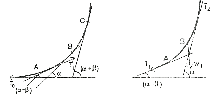
(a) एक भारी डोरी, जिसका घनत्व एक समान नहीं है, दो बिन्दुओं से टँगी हुई है। माना कि T_(1),T_(2),T_(3)T_1, T_2, T_3 क्रमशः कैटिनरी के बीच के बिन्दुओं A,B,CA, B, C पर तनाव हैं, जिन पर इसके क्षैतिज के साथ आनति कोण, सार्व अंतर beta\beta के साथ समांतर श्रेढ़ी में हैं। माना कि डोरी के ABA B तथा BCB C भागों के भार क्रमशः omega_(1)\omega_1 तथा omega_(2)\omega_2 हैं। सिद्ध कीजिए
(i) T_(1),T_(2)T_1, T_2 तथा T_(3)T_3 का हरात्मक माध्य =(3T_(2))/(1+2cos beta)=\frac{3 T_2}{1+2 \cos \beta}
(ii) (T_(1))/(T_(3))=(omega_(1))/(omega_(2))\frac{T_1}{T_3}=\frac{\omega_1}{\omega_2}
A heavy string, which is not of uniform density, is hung up from two points. Let T_(1),T_(2),T_(3)T_1, T_2, T_3 be the tensions at the intermediate points A,B,CA, B, C of the catenary respectively where its inclinations to the horizontal are in arithmetic progression with common difference beta\beta. Let omega_(1)\omega_1 and omega_(2)\omega_2 be the weights of the parts ABA B and BCB C of the string respectively. Prove that
(i) Harmonic mean of T_(1),T_(2)T_1, T_2 and T_(3)=(3T_(2))/(1+2cos beta)T_3=\frac{3 T_2}{1+2 \cos \beta}
(ii) (T_(1))/(T_(3))=(omega_(1))/(omega_(2))\frac{T_1}{T_3}=\frac{\omega_1}{\omega_2}
Answer:
Let OO be the lowest point of the catenary and T_(1),T_(2),T_(3)T_1, T_2, T_3 be the tensions at A,BA, B and CC respectively.
If T_(0)T_0 be the tension at o , then consider the equilibrium of the portion OAO A of the chain.
Using trigonometric identities, we can simplify this to the desired form.
Using the trigonometric identity cos(A)+cos(B)=2cos((A+B)/(2))cos((A-B)/(2))\cos(A) + \cos(B) = 2 \cos\left(\frac{A+B}{2}\right) \cos\left(\frac{A-B}{2}\right), we get:
We aim to prove that (T_(1))/(T_(3))=(omega_(1))/(omega_(2))\frac{T_1}{T_3} = \frac{\omega_1}{\omega_2}.
Using the given equilibrium equations, we can express omega_(1)\omega_1 and omega_(2)\omega_2 in terms of T_(1),T_(2),T_(3)T_1, T_2, T_3 and alpha,beta\alpha, \beta.
Multiply equation (3) by T_(3)T_3 & equation (4) by T_(1)T_1 and subtracting,
We get
Using cos C+cos D=2cos((C+D)/(2))cos((C-D)/(2))\cos C+\cos D=2 \cos \frac{C+D}{2} \cos \frac{C-D}{2}
and sin C+sin D=2sin((C+D)/(2))cos((C-D)/(2))\sin C+\sin D=2 \sin \frac{C+D}{2} \cos \frac{C-D}{2}
6.(b) सभी अन्तर्त्रस्त (शामिल) चरणों को दर्शति हुए समीकरण : (d^(2)y)/(dx^(2))+(tan x-3cos x)(dy)/(dx)+2ycos^(2)x=cos^(4)x\frac{d^2 y}{d x^2}+(\tan x-3 \cos x) \frac{d y}{d x}+2 y \cos ^2 x=\cos ^4 x
को पूर्ण रूप से हल कीजिए ।
Solve the equation: (d^(2)y)/(dx^(2))+(tan x-3cos x)(dy)/(dx)+2ycos^(2)x=cos^(4)x\frac{d^2 y}{d x^2}+(\tan x-3 \cos x) \frac{d y}{d x}+2 y \cos ^2 x=\cos ^4 x
completely by demonstrating all the steps involved.
Answer:
Given equation (d^(2)y)/(dx^(2))+(tan x-3cos x)(dy)/(dx)+2ycos^(2)x=cos^(4)x\frac{d^2 y}{d x^2}+(\tan x-3 \cos x) \frac{d y}{d x}+2 y \cos ^2 x=\cos ^4 x
Compare this equation with (d^(2)y)/(dx^(2))+P(dy)/(dx)+Qy=R\frac{d^2 y}{d x^2}+P \frac{d y}{d x}+Q y=R
We get
{:[P=tan x-3cos x],[Q=2cos^(2)x],[R=cos^(4)x]:}\begin{aligned}
& P=\tan x-3 \cos x \\
& Q=2 \cos ^2 x \\
& R=\cos ^4 x
\end{aligned}
To solve the given differential equation we change the independent variable from xx to zz by choosing zz such that
{:[((dz)/(dx))^(2)=cos^(2)x],[(dz)/(dx)=cos x],[z=sin x]:}\begin{aligned}
& \left(\frac{d z}{d x}\right)^2=\cos ^2 x \\
& \frac{d z}{d x}=\cos x \\
& z=\sin x
\end{aligned}
Now by the substitution z=sin xz=\sin x, the given differential equation is transformed into (d^(2)y)/(dz^(2))+P_(1)(dy)/(dz)+Q_(1)y=R_(1)\frac{d^2 y}{d z^2}+P_1 \frac{d y}{d z}+Q_1 y=R_1
Where
6.(c) int _(C) vec(F)*d vec(r)\int_C \vec{F} \cdot d \vec{r} का मान निकालिए,
जहाँ C,xyC, x y-समतल में एक स्वैच्छिक संवृत वक्र है तथा vec(F)=(-y( hat(i))+x( hat(j)))/(x^(2)+y^(2))\vec{F}=\frac{-y \hat{i}+x \hat{j}}{x^2+y^2} है।
Evaluate int _(C) vec(F)*d vec(r)\int_C \vec{F} \cdot d \vec{r}, where CC is an arbitrary closed curve in the xyx y-plane and vec(F)=(-y( hat(i))+x( hat(j)))/(x^(2)+y^(2))\vec{F}=\frac{-y \hat{i}+x \hat{j}}{x^2+y^2}.
Answer:
To evaluate the line integral int _(C) vec(F)*d vec(r)\int_C \vec{F} \cdot d \vec{r}, where CC is an arbitrary closed curve in the xyxy-plane and vec(F)=(-y( hat(i))+x( hat(j)))/(x^(2)+y^(2))\vec{F}=\frac{-y \hat{i}+x \hat{j}}{x^2+y^2}, we can use the following steps:
Step 1: Check for Conservative Vector Field
First, let’s check if vec(F)\vec{F} is a conservative vector field. A vector field vec(F)=P hat(i)+Q hat(j)\vec{F} = P \hat{i} + Q \hat{j} is conservative if (del P)/(del y)=(del Q)/(del x)\frac{\partial P}{\partial y} = \frac{\partial Q}{\partial x}.
For vec(F)=(-y( hat(i))+x( hat(j)))/(x^(2)+y^(2))\vec{F}=\frac{-y \hat{i}+x \hat{j}}{x^2+y^2}, we have:
To find the partial derivatives, we can use the quotient rule for differentiation, which is (d)/(dx)((u)/(v))=(vu^(‘)-uv^(‘))/(v^(2))\frac{d}{dx} \left( \frac{u}{v} \right) = \frac{vu’ – uv’}{v^2}.
We can integrate these partial derivatives to find f(x,y)f(x, y).
Step 4: Evaluate the Line Integral for a Conservative Field
For a conservative vector field, the line integral over a closed curve CC is zero:
oint_(C) vec(F)*d vec(r)=0\oint_C \vec{F} \cdot d \vec{r} = 0
Therefore, the line integral of vec(F)\vec{F} over any arbitrary closed curve CC in the xyxy-plane is zero.
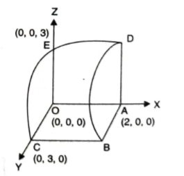
(a) प्रथम अष्टांशक में y^(2)+z^(2)=9y^2+z^2=9 तथा x=2x=2 द्वारा परिबद्ध क्षेत्र पर vec(F)=2x^(2)y hat(i)-y^(2) hat(j)+4xz^(2) hat(k)\vec{F}=2 x^2 y \hat{i}-y^2 \hat{j}+4 x z^2 \hat{k} के लिए गाउस अपसरण प्रमेय को सत्यापित कीजिए ।
Verify Gauss divergence theorem for vec(F)=2x^(2)y hat(i)-y^(2) hat(j)+4xz^(2) hat(k)\vec{F}=2 x^2 y \hat{i}-y^2 \hat{j}+4 x z^2 \hat{k} taken over the region in the first octant bounded by y^(2)+z^(2)=9y^2+z^2=9 and x=2x=2.
Answer:
bar(F)=2x^(2)y hat(i)-y^(2) hat(j)+4xz^(2) hat(k)—-(1)|”given”\overline{\mathrm{F}}=2 x^2 y \hat{i}-y^2 \hat{j}+4 x z^2 \hat{k}—-(1) | \text{given}
{:[div bar(F)=(( hat(i))(del)/(del x)+( hat(j))(del)/(del y)+( hat(k))(del)/(del z))*(2x^(2)y( hat(i))-y^(2)( hat(j))+4xz^(2)( hat(k)))=4xy-2y+8xz],[:.quad∭_(V)div bar(F)dV=int_(x=0)^(2)int_(y=0)^(3)int_(z=0)^(sqrt(9-y^(2)))(4xy-2y+8xz)dzdydx],[=int_(x=0)^(2)int_(y=0)^(3)[4xysqrt(9-y^(2))-2ysqrt(9-y^(2))+4x(9-y^(2))]dydx],[=int_(x=0)^(2)[(-4x)/(2)*(2)/(3)(9-y^(2))^(3//2)+(2)/(3)(9-y^(2))^(3//2)+36 xy-(4)/(3)xy^(3)]_(0)^(3)dx],[=int_(x=0)^(2)(108 x-18 x)dx=(54x^(2)-18 x)_(0)^(2)],[=216-36=180—-(2)]:}\begin{aligned}
\operatorname{div} \overline{\mathrm{F}} & =\left(\hat{i} \frac{\partial}{\partial x}+\hat{j} \frac{\partial}{\partial y}+\hat{k} \frac{\partial}{\partial z}\right) \cdot\left(2 x^2 y \hat{i}-y^2 \hat{j}+4 x z^2 \hat{k}\right)=4 x y-2 y+8 x z \\
\therefore \quad \iiint_{\mathrm{V}} \operatorname{div} \overline{\mathrm{F}} d \mathrm{~V} & =\int_{x=0}^2 \int_{y=0}^3 \int_{z=0}^{\sqrt{9-y^2}}(4 x y-2 y+8 x z) d z d y d x \\
& =\int_{x=0}^2 \int_{y=0}^3\left[4 x y \sqrt{9-y^2}-2 y \sqrt{9-y^2}+4 x\left(9-y^2\right)\right] d y d x \\
& =\int_{x=0}^2\left[\frac{-4 x}{2} \cdot \frac{2}{3}\left(9-y^2\right)^{3 / 2}+\frac{2}{3}\left(9-y^2\right)^{3 / 2}+36 x y-\frac{4}{3} x y^3\right]_0^3 d x\\
& =\int_{x=0}^2(108 x-18 x) d x=\left(54 x^2-18 x\right)_0^2 \\
& =216-36=180—-(2)
\end{aligned}
To evaluate ∬_(S) bar(F)* hat(n)dS\iint_{\mathrm{S}} \overline{\mathrm{F}} \cdot \hat{n} d \mathrm{~S}
The surface SS consists of five parts.
∬_(S) bar(F)* hat(n)dS=∬_(OABC) bar(F)* hat(n)dS+∬_(OCE) bar(F)* hat(n)dS+∬_(OADE) bar(F)* hat(n)dS+∬_(ABD) bar(F)* hat(n)dS+∬_(BDEC) bar(F)* hat(n)dS—-(3)\iint_{\mathrm{S}} \overline{\mathrm{F}} \cdot \hat{n} d \mathrm{~S}=\iint_{\mathrm{OABC}} \overline{\mathrm{F}} \cdot \hat{n} d \mathrm{~S}+\iint_{\mathrm{OCE}} \overline{\mathrm{F}} \cdot \hat{n} d \mathrm{~S}+\iint_{\mathrm{OADE}} \overline{\mathrm{F}} \cdot \hat{n} d \mathrm{~S}+\iint_{\mathrm{ABD}} \overline{\mathrm{F}} \cdot \hat{n} d \mathrm{~S}+\iint_{\mathrm{BDEC}} \overline{\mathrm{F}} \cdot \hat{n} d \mathrm{~S}—-(3)
Over the surface OABC, z=0,dz=0, hat(n)=- hat(k),dS=dxdyz=0, d z=0, \hat{n}=-\hat{k}, d \mathrm{~S}=d x d y
∬_(OABC) bar(F), hat(n)dS=∬(2x^(2)y( hat(i))-y^(2)( hat(j)))(- hat(k))dxdy=0—-(4)\iint_{\mathrm{OABC}} \overline{\mathrm{F}}, \hat{n} d \mathrm{~S}=\iint\left(2 x^2 y \hat{i}-y^2 \hat{j}\right)(-\hat{k}) d x d y=0—-(4)
Over the surface OCE, x=0,dx=0, hat(n)=- hat(i),dS=dydzx=0, d x=0, \hat{n}=-\hat{i}, d \mathrm{~S}=d y d z
∬_(OCE) bar(F)* hat(n)dS=∬(-y^(2)( hat(j)))*(- hat(i))dydz=0—-(5)\iint_{\mathrm{OCE}} \overline{\mathrm{F}} \cdot \hat{n} d \mathrm{~S}=\iint\left(-y^2 \hat{j}\right) \cdot(-\hat{i}) d y d z=0—-(5)
Over the surface OADE, y=0,dy=0, hat(n)=- hat(j),d8=dzdxy=0, d y=0, \hat{n}=-\hat{j}, d 8=d z d x
∬_(ODE) bar(F), hat(n)dS=∬(4xz^(2)( hat(k))),(- hat(j))dzdx=0—-(6)\iint_{\mathrm{ODE}} \overline{\mathrm{F}}, \hat{n} d \mathrm{~S}=\iint\left(4 x z^2 \hat{k}\right),(-\hat{j}) d z d x=0—-(6)
Over the surface ABD, x=2,dx=0, hat(A)= hat(f),d8=dydzx=2, d x=0, \hat{A}=\hat{f}, d \mathbf{8}=d y d z
{:[∬_(ABC) bar(F)* hat(n)dS=∬(8y( hat(i))-y^(2)( hat(j))+8z^(2)( hat(hat(h))))”,” hat(ı)dydz],[=int_(z=0)^(3)int_(y=0)^(sqrt(9-z^(3)))8ydydz=int_(z=0)^(3)(4y^(2))_(0)^(sqrt(9-z^(3)))dz],[=4int_(z=0)^(3)(9-z^(2))dz=4(9z-(z^(3))/(3))_(0)^(3)=4(27-9)=72—-(7)]:}\begin{aligned}
\iint_{\mathrm{ABC}} \overline{\mathrm{F}} \cdot \hat{\mathrm{n}} d \mathrm{~S} & =\iint\left(8 y \hat{i}-y^2 \hat{j}+8 z^2 \hat{\hat{h}}\right), \hat{\imath} d y d z \\
& =\int_{z=0}^3 \int_{y=0}^{\sqrt{9-z^3}} 8 y d y d z=\int_{z=0}^3\left(4 y^2\right)_0^{\sqrt{9-z^3}} d z \\
& =4 \int_{z=0}^3\left(9-z^2\right) d z=4\left(9 z-\frac{z^3}{3}\right)_0^3=4(27-9)=72—-(7)
\end{aligned}
{:[∬_(BDEC) bar(F)* hat(n)dS=∬_(BDEC)(2x^(2)y( hat(i))-y^(2)( hat(j))+4xz^(2)( hat(k)))*((y( hat(j))+z( hat(k)))/(3))(dxdy)/((( hat(n))*( hat(k))))],[=∬_(BDEC)((-y^(3)+4xz^(3)))/(3)(dxdy)/(((z)/(3)))=int_(x=0)^(2)int_(y=0)^(3)(-(y^(3))/(z)+4xz^(2))dxdy],[=int_(x=0)^(2)int_(y=0)^(pi//2)[(-27sin^(3)theta)/(3cos theta)+4x(9cos^(2)theta)]3cos theta d theta dx],[=int_(x=0)^(2)int_(y=0)^(pi//2)(-27sin^(3)theta+108 xcos^(3)theta)d theta dx],[=int_(x=0)^(2)((-54)/(3)+108 x xx(2)/(3))dx=int_(0)^(2)(-18+72 x)dx],[=(-18 x+36x^(2))_(0)^(2)=108—-(8)]:}\begin{aligned}
\iint_{\mathrm{BDEC}} \overline{\mathrm{F}} \cdot \hat{n} d \mathrm{~S} & =\iint_{\mathrm{BDEC}}\left(2 x^2 y \hat{i}-y^2 \hat{j}+4 x z^2 \hat{k}\right) \cdot\left(\frac{y \hat{j}+z \hat{k}}{3}\right) \frac{d x d y}{(\hat{n} \cdot \hat{k})} \\
& =\iint_{\mathrm{BDEC}} \frac{\left(-y^3+4 x z^3\right)}{3} \frac{d x d y}{\left(\frac{z}{3}\right)}=\int_{x=0}^2 \int_{y=0}^3\left(-\frac{y^3}{z}+4 x z^2\right) d x d y \\
& =\int_{x=0}^2 \int_{y=0}^{\pi / 2}\left[\frac{-27 \sin ^3 \theta}{3 \cos \theta}+4 x\left(9 \cos ^2 \theta\right)\right] 3 \cos \theta d \theta d x \\
& =\int_{x=0}^2 \int_{y=0}^{\pi / 2}\left(-27 \sin ^3 \theta+108 x \cos ^3 \theta\right) d \theta d x \\
& =\int_{x=0}^2\left(\frac{-54}{3}+108 x \times \frac{2}{3}\right) d x=\int_0^2(-18+72 x) d x \\
& =\left(-18 x+36 x^2\right)_0^2=108—-(8)
\end{aligned}
From eqn. (3),
∬_(S) vec(F)* hat(n)dS=0+0+0+72+108=180—-(9)\iint_{\mathrm{S}} \overrightarrow{\mathrm{F}} \cdot \hat{n} d \mathrm{~S}=0+0+0+72+108=180—-(9)
From results (2) and (8), it is clear that
∬_(B) vec(F)* hat(n)dS=∭_(V)div vec(F)dV\iint_{\mathrm{B}} \overrightarrow{\mathrm{F}} \cdot \hat{n} d \mathbf{S}=\iiint_{\mathrm{V}} \operatorname{div} \overrightarrow{\mathrm{F}} d \mathrm{~V}
Hence, Gauss’ divergence theorem is verified.
7.(b) अवकल समीकरण :
y^(2)log y=xy(dy)/(dx)+((dy)/(dx))^(2)y^2 \log y=x y \frac{d y}{d x}+\left(\frac{d y}{d x}\right)^2
के सभी सम्भव हल ज्ञात कीजिए ।
Find all possible solutions of the differential equation :
{:[log _(e)p=log _(e)y+log _(e)c],[log _(e)p=log _(e)yc],[p=cy]:}\begin{aligned}
\log _e p & =\log _e y+\log _e c \\
\log _e p & =\log _e y c \\
p & =c y
\end{aligned}
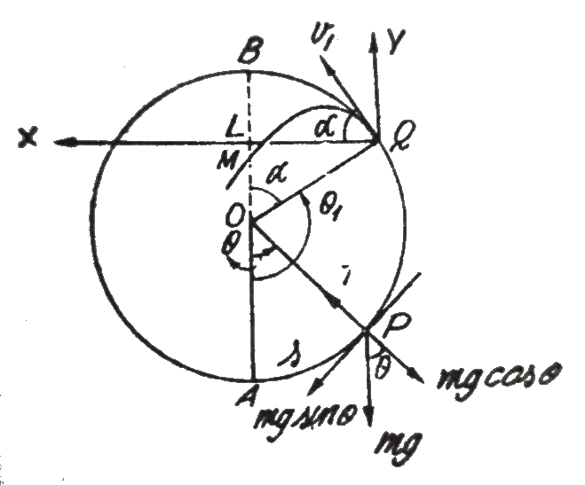
(c) एक भारी कण aa लम्बाई की अवितान्य डोरी से एक स्थिर बिन्दु से टँगा है तथा sqrt(2gh)\sqrt{2 g h} वेग से क्षैतिज दिशा में प्रक्षेपित किया जाता है । यदि (5a)/(2) > h > a\frac{5 a}{2}>h>a है, तो सिद्ध कीजिए कि प्रक्षेपण बिन्दु से (1)/(3)(a+2h)\frac{1}{3}(a+2 h) ऊँचाई पहुँचने पर कण की वृत्तीय गति समाप्त हो जाती है । यह भी सिद्ध कीजिए कि उस कण द्वारा प्रक्षेपण बिंदु से ऊपर प्राप्य अधिकतम ऊँचाई ((4a-h)(a+2h)^(2))/(27a^(2))\frac{(4 a-h)(a+2 h)^2}{27 a^2} है ।
A heavy particle hangs by an inextensible string of length aa from a fixed point and is then projected horizontally with a velocity sqrt(2gh)\sqrt{2 g h}.
If (5a)/(2) > h > a\frac{5 a}{2}>h>a, then prove that the circular motion ceases when the particle has reached the height (1)/(3)(a+2h)\frac{1}{3}(a+2 h) from the point of projection. Also, prove that the greatest height ever reached by the particle above the point of projection is ((4a-h)(a+2h)^(2))/(27a^(2))\frac{(4 a-h)(a+2 h)^2}{27 a^2}.
Answer:
Let a particle of mass m\mathrm{m} be attached to one end of a string of length a whole other end is fixed at O\mathrm{O}. The particle is projected horizontally with a velocity u=sqrt(2gh)u=\sqrt{2 g h} from AA.
If P\mathrm{P} is the portion of the particle at time t such that angle of AOP=thetaA O P=\theta and arc AP=s\operatorname{arc} A P=s,
Then the equations of the motion of the particle are m(d^(2)s)/(dt^(2))=-mg sin theta rarr(1)m \frac{\mathbf{d}^2 s}{\mathbf{d} t^2}=-m g \sin \theta \rightarrow(1)
And m(v^(2))/(a)=T-mg cos theta rarr(2)m \frac{v^2}{a}=T-m g \cos \theta \rightarrow(2)
Also s=a theta rarr(3)s=a \theta \rightarrow(3)
From (1) and (3), we have a(d^(2)theta)/(dt^(2))=-g sin thetaa \frac{\mathbf{d}^2 \theta}{\mathbf{d} t^2}=-g \sin \theta
Multiplying both sides by 2a(dtheta)/(dt)2 a \frac{\mathbf{d} \theta}{\mathbf{d} t} and integrating, we have
v^(2)=(a(dtheta)/(dt))^(2)=2ag cos theta+Av^2=\left(a \frac{\mathbf{d} \theta}{\mathbf{d} t}\right)^2=2 a g \cos \theta+A
But at the point A, theta=0\theta=0 and v=u=sqrt(2gh)v=u=\sqrt{2 g h}
{:[A=2gh-2ag],[v^(2)=2ag cos theta+2gh-2ag rarr(4)]:}\begin{aligned}
& A=2 g h-2 a g \\
& v^2=2 a g \cos \theta+2 g h-2 a g \rightarrow(4)
\end{aligned}
From (2) and (4), we have
T=(m)/(a)(v^(2)+ag cos theta)=(m)/(a)(3ag cos theta+2gh-2ag)T=\frac{m}{a}\left(v^2+a g \cos \theta\right)=\frac{m}{a}(3 a g \cos \theta+2 g h-2 a g)
If the particle leaves the circular path at Q\mathrm{Q} where theta=theta_(1)\theta=\theta_1, then T=0T=0 when theta=theta_(1)\theta=\theta_1
0=(m)/(a)(3ag cos theta_(1)+2gh-2ag)=>cos theta_(1)=-(2h-2a)/(3a)0=\frac{m}{a}\left(3 a g \cos \theta_1+2 g h-2 a g\right) \Rightarrow \cos \theta_1=-\frac{2 h-2 a}{3 a}
Since (5)/(2)a > h > a\frac{5}{2} a>h>a that is 5a > 2h > 2a5 a>2 h>2 a, therefore cos theta_(1)\cos \theta_1 is negative and its absolute value is < 1<1. so theta_(1)\theta_1 is real and (1)/(2)pi < theta_(1) < pi\frac{1}{2} \pi<\theta_1<\pi
Thus, the particle leaves the circular path at QQ before arriving at the highest point
Height of the point Q\mathrm{Q} above A=AL=AO+OL=a+a cos(pi-theta_(1))\mathrm{A}=A L=A O+O L=a+a \cos \left(\pi-\theta_1\right)
That is the particle leaves the circular path when it has reached a height (1)/(3)(a+2h)\frac{1}{3}(a+2 h) above the point of projection.
If v_(1)v_1 is the velocity of the particle at the point QQ, then from (4), we have
{:[v_(1)^(2)=2ag cos theta_(1)+2gh-2ag],[=-2ag((2h-2a)/(3a))+2g(h-a)],[=2g(h-a)(1-(2)/(3))=(2)/(3)g(h-a)]:}\begin{aligned}
& v_1^2=2 a g \cos \theta_1+2 g h-2 a g \\
& =-2 a g \frac{2 h-2 a}{3 a}+2 g(h-a) \\
& =2 g(h-a)\left(1-\frac{2}{3}\right)=\frac{2}{3} g(h-a)
\end{aligned}
If angle of LOQ =alpha=\alpha, then alpha=pi-theta_(1)\alpha=\pi-\theta_1
cos alpha=cos(pi-theta_(1))=-cos theta_(1)=(2(h-a))/(3a)\cos \alpha=\cos \left(\pi-\theta_1\right)=-\cos \theta_1=\frac{2(h-a)}{3 a}
Thus the particle leaves the circular path at the point Q\mathrm{Q} with velocity v_(1)=sqrt({(2)/(3)g(h-a)})v_1=\sqrt{\left\{\frac{2}{3} g(h-a)\right\}} at an angle alpha=cos^(-1){(2(h-d))/(3a)}\alpha=\cos ^{-1}\left\{\frac{2(h-d)}{3 a}\right\} to the horizontal and will subsequently describe a parabolic path.
(a)(i) संनाभि शांकव कुल (x^(2))/(a^(2)+lambda)+(y^(2))/(b^(2)+lambda)=1;a > b > 0\frac{x^2}{a^2+\lambda}+\frac{y^2}{b^2+\lambda}=1 ; a>b>0 अचर हैं तथा lambda\lambda एक प्राचल है,
के लंबकोणीय संछेदी ज्ञात कीजिए । दर्शाइए कि दिया गया वक्र-कुल स्वलांबिक है।
Find the orthogonal trajectories of the family of confocal conics (x^(2))/(a^(2)+lambda)+(y^(2))/(b^(2)+lambda)=1;quad a > b > 0\frac{x^2}{a^2+\lambda}+\frac{y^2}{b^2+\lambda}=1 ; \quad a>b>0 are constants and lambda\lambda is a parameter. Show that the given family of curves is self orthogonal.
Answer:
Given (x^(2))/(a^(2)+lambda)+(y^(2))/(b^(2)+lambda)=1rarr(1)\frac{x^2}{a^2+\lambda}+\frac{y^2}{b^2+\lambda}=1 \rightarrow(1)
Differentiating, (2x)/(a^(2)+lambda)+(2y)/(b^(2)+lambda)(dy)/(dx)=0\frac{2 x}{a^2+\lambda}+\frac{2 y}{b^2+\lambda} \frac{\mathbf{d} y}{\mathbf{d} x}=0 or lambda(x+y(dy)/(dx))=-(b^(2)x+a^(2)y(dy)/(dx))\lambda\left(x+y \frac{\mathbf{d} y}{\mathbf{d} x}\right)=-\left(b^2 x+a^2 y \frac{\mathbf{d} y}{\mathbf{d} x}\right)
Which is the differential equation of the family (1), Replacing (dy)/(dx)by(-(dx)/(dy))\frac{\mathbf{d} y}{\mathbf{d} x} b y\left(-\frac{\mathbf{d} x}{\mathbf{d} y}\right) in (2), the differential equation of the required orthogonal trajectories is
Which is the same as the differential equation (2) of the given family of curves (1).
Hence, the system of the given curve (1) is self orthogonal, that is each member of the given family of curves intersects its own members orthogonally.
(a)(ii) अवकल समीकरण : x^(2)(d^(2)y)/(dx^(2))-2x(1+x)(dy)/(dx)+2(1+x)y=0x^2 \frac{d^2 y}{d x^2}-2 x(1+x) \frac{d y}{d x}+2(1+x) y=0 का व्यापक हल ज्ञात कीजिए । अतः अवकल समीकरण : x^(2)(d^(2)y)/(dx^(2))-2x(1+x)(dy)/(dx)+2(1+x)y=x^(3)x^2 \frac{d^2 y}{d x^2}-2 x(1+x) \frac{d y}{d x}+2(1+x) y=x^3 को प्राचल विचरण विधि द्वारा हल कीजिए ।
Find the general solution of the differential equation : x^(2)(d^(2)y)/(dx^(2))-2x(1+x)(dy)/(dx)+2(1+x)y=0x^2 \frac{d^2 y}{d x^2}-2 x(1+x) \frac{d y}{d x}+2(1+x) y=0.
Hence, solve the differential equation: x^(2)(d^(2)y)/(dx^(2))-2x(1+x)(dy)/(dx)+2(1+x)y=x^(3)x^2 \frac{d^2 y}{d x^2}-2 x(1+x) \frac{d y}{d x}+2(1+x) y=x^3 by the method of variation of parameters.
Answer:
Important Result:
(i) y=xy=x is a solution if P+Qx=0P+Q x=0.
(ii) y=x^(2)y=x^2 is a solution if 2+2Px+Qx^(2)=02+2 \mathrm{Px}+\mathrm{Qx}^2=0.
(i) y=e^(x)y=e^x is a part of C.F. if 1+P+Q=01+P+Q=0.
(ii) y=e^(-x)y=e^{-x} is a part of C.F. if 1-P+Q=01-P+Q=0.
(iii) y=e^(m_(x))y=e^{m_x} is a part of C.F. if m^(2)+mP+Q=0m^2+m P+Q=0.
(iv) y=xy=x is a part of C.F. if P+Qx=0P+Q x=0.
(v) y=x^(2)y=x^2 is a pait of C.F. if 2+2Px+Qx^(2)=02+2 P x+Q x^2=0.
(vi) y=x^(m)y=x^m is a part of C.F. if m(m-1)+Pmx+Qx^(2)=0m(m-1)+P m x+Q x^2=0.
Very Important. If in a linear differential equation
the sum of the coefficients of d^(2)y//dx^(2),dy//dxd^2 y / d x^2, d y / d x and yy is zero i.e., if A+B+C=0A+B+C=0, then y=e^(x)y=e^x is a part of the C.F. of the solution of the differential equation.
Solved Examples
{:[y=vx],[y=(-x^(2))/(2)+(c_(1)xe^(2x))/(2)+xc_(2)]:}\begin{aligned}
& y=v x \\
& y=\frac{-x^2}{2}+\frac{c_1 x e^{2 x}}{2}+x c_2
\end{aligned}
8.(b) द्रव्यमान mm का एक कण, जो की प्रक्षेपण बिन्दु से वेग uu के साथ क्षैतिज दिशा के साथ theta\theta कोण बनाने वाली दिशा में प्रक्षेपण बिन्दु से गुजरने वाले ऊर्ध्वाधर समतल में प्रक्षेपित किया जाता है, उसकी गति तथा पथ का वर्णन कीजिए । यदि कणों को उसी बिन्दु से उसी ऊर्ध्वाधर समतल में वेग 4sqrtg4 \sqrt{g} के साथ प्रक्षेपित किया जाता है, तो उनके पथों के शीर्षों के बिन्दुपथ को भी निर्धारित कीजिए ।
Describe the motion and path of a particle of mass mm which is projected in a vertical plane through a point of projection with velocity uu in a direction making an angle theta\theta with the horizontal direction. Further, if particles are projected from that point in the same vertical plane with velocity 4sqrtg4 \sqrt{g}, then determine the locus of vertices of their paths.
Answer:
Given Problem
A particle of mass mm is projected in a vertical plane with an initial velocity uu at an angle theta\theta with the horizontal direction.
Equations of Motion
Given the particle with the mass m\mathrm{m}, is projected from the point in the vertical plane with velocity u\mathrm{u},
Which is projected in a vertical plane through a point of projection with velocity u\mathrm{u} in a direction making an angle theta\theta with horizontal direction.
The initial velocity theta\theta
Then mx^(¨)=0m \ddot{x}=0 and my^(¨)=-mg=>y^(¨)=-gm \ddot{y}=-m g \Rightarrow \ddot{y}=-g
{:[y^(˙)=-gt+B” when “t=0;u sin theta=B],[y^(˙)=-gt+u sin theta]:}\begin{aligned}
&\dot{y}=-g t+B \text { when } t=0 ; u \sin \theta=B \\
& \dot{y}=-g t+u \sin \theta
\end{aligned}
By Integrating
{:[y=-(gt^(2))/(2)+u sin theta t+B^(‘)” when “t=0”,”y=0;B^(‘)=0],[y=u sin theta t-(gt^(2))/(2)]:}\begin{aligned}
& y=-\frac{g t^2}{2}+u \sin \theta t+B^{\prime} \text { when } t=0, y=0 ; B^{\prime}=0 \\
& y=u \sin \theta t-\frac{g t^2}{2}
\end{aligned}
Then mx^(¨)=0,x^(¨)=0,x^(˙)=cm \ddot{x}=0, \ddot{x}=0, \dot{x}=c
Path and Trajectory
{:x=u cos theta t:}\begin{aligned}
& x=u \cos \theta t
\end{aligned}
By eliminating t we get path and trajectory
Here t=(x)/(u cos theta)t=\frac{x}{u \cos \theta}
Therefore, path of trajectory; y=x tan theta-(gx^(2))/(2u^(2)cos^(2)theta)y=x \tan \theta-\frac{g x^2}{2 u^2 \cos ^2 \theta}
Multiply both sides by -(2u^(2)cos^(2)alpha)/(g)-\frac{2 u^2 \cos ^2 \alpha}{g}
By rearranging we get (x-(u^(2)sin alpha cos alpha)/(g))=(-2a^(2)cos^(2)alpha)/(g)(y-(u^(2)sin^(2)alpha)/(2g))\left(x-\frac{u^2 \sin \alpha \cos \alpha}{g}\right)=\frac{-2 a^2 \cos ^2 \alpha}{g}\left(y-\frac{u^2 \sin ^2 \alpha}{2 g}\right)
This equation describes the locus of the vertices of the paths when u=4sqrtgu = 4 \sqrt{g}.
(c) स्टोक्स प्रमेय का उपयोग करते हुए ∬_(S)(grad xx vec(F))* hat(n)dS\iint_S(\nabla \times \vec{F}) \cdot \hat{n} d S का मान निकालिए, जहाँ पर vec(F)=(x^(2)+y-4) hat(i)+3xy hat(j)+(2xy+z^(2)) hat(k)\vec{F}=\left(x^2+y-4\right) \hat{i}+3 x y \hat{j}+\left(2 x y+z^2\right) \hat{k} तथा SS, परवलयज z=4-(x^(2)+y^(2))z=4-\left(x^2+y^2\right) का xyx y-समतल से ऊपर का पृष्ठ है। यहाँ hat(n),S\hat{n}, S पर एकक बहिर्मुखी अभिलंब सदिश है ।
Using Stokes’ theorem, evaluate ∬_(S)(grad xx vec(F))* hat(n)dS\iint_S(\nabla \times \vec{F}) \cdot \hat{n} d S, where vec(F)=(x^(2)+y-4) hat(i)+3xy hat(j)+(2xy+z^(2)) hat(k)\vec{F}=\left(x^2+y-4\right) \hat{i}+3 x y \hat{j}+\left(2 x y+z^2\right) \hat{k} and SS is the surface of the paraboloid z=4-(x^(2)+y^(2))z=4-\left(x^2+y^2\right) above the xyx y-plane. Here, hat(n)\hat{n} is the unit outward normal vector on SS.
Answer:
Stoke’s theorem is
int_(C) bar(F)*d bar(r)=∬_(S)curl bar(F)* hat(n)dS\int_{\mathrm{C}} \overline{\mathrm{F}} \cdot d \bar{r}=\iint_{\mathrm{S}} \operatorname{curl} \overline{\mathrm{F}} \cdot \hat{n} d \mathrm{~S}
where C\mathrm{C} is the circle, x^(2)+y^(2)=4,z=0x^2+y^2=4, z=0
Also, quad bar(F)*d bar(r)=[(x^(2)+y-4)( hat(i))+3xy( hat(j))+(2xz+z^(2))( hat(k))]*(dx hat(i)+dy hat(j)+dz hat(k))\quad \overline{\mathrm{F}} \cdot d \bar{r}=\left[\left(x^2+y-4\right) \hat{i}+3 x y \hat{j}+\left(2 x z+z^2\right) \hat{k}\right] \cdot(d x \hat{i}+d y \hat{j}+d z \hat{k})
=(x^(2)+y-4)dx+3xydy+(2xz+z^(2))dz=\left(x^2+y-4\right) d x+3 x y d y+\left(2 x z+z^2\right) d z
On the circle
{:[z=0″,”,:.dz=0],[x=2cos phi”,”,:.dx=-2sin phi d phi],[y=2sin phi”,”,:.dy=2cos phi” d “phi]:}\begin{array}{ll}
z=0, & \therefore d z=0 \\
x=2 \cos \phi, & \therefore d x=-2 \sin \phi d \phi \\
y=2 \sin \phi, & \therefore d y=2 \cos \phi \text { d } \phi
\end{array}
{:[:.quadint _(C) bar(F)*d bar(r){:=int _(C)[x^(2)+y-4)dx+3xydy]],[=int_(0)^(2pi)(4cos^(2)phi+2sin phi-4)(-2sin phi d phi)+3(2cosphi)(2sinphi)(2cosphid phi)],[=int_(0)^(2pi)(-8cos^(2)phi sin phi-4sin^(2)phi+8sin^(2)phi+24cos^(2)phi sin phi)d phi],[=int_(0)^(2pi)(16cos^(2)phi sin phi-4sin^(2)phi+8sin phi)d phi],[=-4int_(0)^(2pi)sin^(2)phi d phi=-4xx4int_(0)^(pi//2)sin^(2)phi d phi=-16((1)/(2)(pi)/(2))=-4pi]:}\begin{aligned}
\therefore \quad \int_C \bar{F} \cdot d \bar{r} & \left.=\int_C\left[x^2+y-4\right) d x+3 x y d y\right] \\
& =\int_0^{2 \pi}\left(4 \cos ^2 \phi+2 \sin \phi-4\right)(-2 \sin \phi d \phi) +3\left(2\:cos\:\phi \right)\left(2\:sin\:\phi \right)\left(2\:cos\:\phi \:d\phi \right)\\
& =\int_0^{2 \pi}\left(-8 \cos ^2 \phi \sin \phi-4 \sin ^2 \phi+8 \sin ^2 \phi+24 \cos ^2 \phi \sin \phi\right) d \phi \\
& =\int_0^{2 \pi}\left(16 \cos ^2 \phi \sin \phi-4 \sin ^2 \phi+8 \sin \phi\right) d \phi \\
& =-4 \int_0^{2 \pi} \sin ^2 \phi d \phi=-4 \times 4 \int_0^{\pi / 2} \sin ^2 \phi d \phi=-16\left(\frac{1}{2} \frac{\pi}{2}\right)=-4 \pi
\end{aligned}