Free UPSC Mathematics Optional Paper-1 2022 Solutions: View Online | UPSC Maths Solution | IAS Maths Solution

July 12, 2025ByAbstract Classes

खण्ड A
SECTION A

Question:-01 (a) सिद्ध कीजिए कि

n

विमीय सदिश समष्टि

V

के लिए

n

रैखिकत: स्वतंत्र सदिशों का कोई भी समुच्चय

V

के लिए एक आधार बनाता है ।

Question:-01 (a) Prove that any set of

n

linearly independent vectors in a vector space

V

of dimension

n

constitutes a basis for

V

Answer:

To prove that any set of

n

linearly independent vectors in a vector space

V

of dimension

n

constitutes a basis for

V

, we need to show two things:

The set spans $V$ .
The set is linearly independent.

Given:

A vector space $V$ of dimension $n$ .
A set $S = {v_{1}, v_{2}, \dots, v_{n}}$ of $n$ linearly independent vectors in $V$ .

Proof:

Step 1: $S$ is Linearly Independent (Given)

We are given that

S

is a set of

n

linearly independent vectors. Therefore, no vector in

S

can be written as a linear combination of the other vectors in

S

Step 2: $S$ Spans $V$

To show that

S

spans

V

, we need to show that any vector

w

V

can be written as a linear combination of vectors in

S

Let’s consider another basis

B

for

V

. Since

V

has dimension

n

B

contains exactly

n

vectors. We can write

w

as a linear combination of vectors in

B

w = c_{1} b_{1} + c_{2} b_{2} + \dots + c_{n} b_{n}

Now, each

b_{i}

can also be written as a linear combination of vectors in

S

because

S

and

B

are both bases for

V

b_{i} = a_{i 1} v_{1} + a_{i 2} v_{2} + \dots + a_{i n} v_{n}

Substituting this into the equation for

w

, we get:

w = \sum_{i = 1}^{n} c_{i} (a_{i 1} v_{1} + a_{i 2} v_{2} + \dots + a_{i n} v_{n})

Simplifying, we find that

w

can indeed be written as a linear combination of vectors in

S

, proving that

S

spans

V

Conclusion

Since

S

is both linearly independent and spans

V

, it constitutes a basis for

V

Thus, we have proven that any set of

n

linearly independent vectors in a vector space

V

of dimension

n

constitutes a basis for

V

Question:-01 (b) माना

T : R^{2} \to R^{3}

एक रैखिक रूपांतरण, ऐसा है कि

T (\begin{array}{l} 1 \\ 0 \end{array}) = (\begin{array}{l} 1 \\ 2 \\ 3 \end{array})

तथा

T (\begin{array}{l} 1 \\ 1 \end{array}) = (\begin{array}{r} - 3 \\ 2 \\ 8 \end{array})

है ।

T (\begin{array}{l} 2 \\ 4 \end{array})

को ज्ञात कीजिए ।

Question:-01(b) Let

T : R^{2} \to R^{3}

be a linear transformation such that

T (\begin{array}{l} 1 \\ 0 \end{array}) = (\begin{array}{l} 1 \\ 2 \\ 3 \end{array})

and

T (\begin{array}{l} 1 \\ 1 \end{array}) = (\begin{array}{r} - 3 \\ 2 \\ 8 \end{array})

. Find

T (\begin{array}{l} 2 \\ 4 \end{array})

Answer:

Introduction: In this problem, we are given a linear transformation

T : R^{2} \to R^{3}

and are asked to find the image of a vector under this transformation. We are given the images of two vectors under

T

and will use this information along with the linearity property of the transformation to find the desired image.
Assumptions: We assume that

T

is a linear transformation.
Definition:

Linear Transformation: A function $T : V \to W$ between two vector spaces $V$ and $W$ is called a linear transformation if for all vectors $u, v \in V$ and scalars $c$ , the following conditions hold:
a. $T (u + v) = T (u) + T (v)$
b. $T (c u) = c T (u)$
Method/Approach: To solve this problem, we will first express the given vector as a linear combination of the two given vectors. Then, we will use the linearity property of the transformation to find the image of the given vector under the transformation $T$ .
Work/Calculations: The calculations have already been provided in the original answer. I’ll restate them here for clarity:
Represent the vector $(\begin{matrix} 2 \\ 4 \end{matrix})$ as a linear combination of the given vectors:

(\begin{array}{l} 2 \\ 4 \end{array}) = a (\begin{array}{l} 1 \\ 0 \end{array}) + b (\begin{array}{l} 1 \\ 1 \end{array})

Solve for $a$ and $b$ :

\begin{aligned} 2 = a + b \\ 4 = 0 + b \end{aligned}

Find $a = - 2$ and $b = 4$ and write the linear combination:

(\begin{array}{l} 2 \\ 4 \end{array}) = - 2 (\begin{array}{l} 1 \\ 0 \end{array}) + 4 (\begin{array}{l} 1 \\ 1 \end{array})

Apply the linear transformation $T$ :

T (\begin{array}{l} 2 \\ 4 \end{array}) = - 2 T (\begin{array}{l} 1 \\ 0 \end{array}) + 4 T (\begin{array}{l} 1 \\ 1 \end{array})

Use the given values for the transformation, perform scalar multiplication and vector addition:

\begin{aligned} T (\begin{matrix} 2 \\ 4 \end{matrix}) = (\begin{matrix} - 2 \\ - 4 \\ - 6 \end{matrix}) + (\begin{array}{c} - 12 \\ 8 \\ 32 \end{array}) = (\begin{array}{c} - 14 \\ 4 \\ 26 \end{array}) \\ Thus, T (\begin{matrix} 2 \\ 4 \end{matrix}) = (\begin{array}{c} - 14 \\ 4 \\ 26 \end{array}) . \end{aligned}

Conclusion: In this problem, we found the image of the vector

(\begin{matrix} 2 \\ 4 \end{matrix})

under the linear transformation

T : R^{2} \to R^{3}

. We expressed the given vector as a linear combination of the two given vectors and used the linearity property of the transformation to find the image.
The image of the given vector under the transformation

T

(\begin{matrix} - 14 \\ 4 \\ 26 \end{matrix})

Question:-01(c)

lim_{x \to \infty} {(e^{x} + x)}^{\frac{1}{x}}

का मान निकालिए ।

Question:-01(c) Evaluate

lim_{x \to \infty} {(e^{x} + x)}^{\frac{1}{x}}

Answer:

Introduction: In this problem, we are asked to evaluate the limit

lim_{x \to \infty} {(e^{x} + x)}^{\frac{1}{x}}

. The expression presents an indeterminate form of type

1^{\infty}

x

approaches infinity. We will use the natural logarithm and L’Hôpital’s rule to resolve this indeterminate form and find the limit.
Assumptions: None.
Definition: Indeterminate form refers to an expression involving limits whose behavior cannot be determined solely based on the behavior of the individual parts of the expression.
Theorem: L’Hôpital’s Rule states that if

lim_{x \to c} \frac{f (x)}{g (x)}

is an indeterminate form of type

\frac{0}{0}

\frac{\infty}{\infty}

, and

f^{'} (x)

and

g^{'} (x)

exist and are continuous in an open interval containing

c

(except possibly at

c

, and

lim_{x \to c} \frac{f^{'} (x)}{g^{'} (x)}

exists or equals

\pm \infty

, then

lim_{x \to c} \frac{f (x)}{g (x)} = lim_{x \to c} \frac{f^{'} (x)}{g^{'} (x)}

.
Method/Approach: The steps in your answer are correct, and I will restate them briefly:

Recognize the indeterminate form of type $1^{\infty}$ .
Use the natural logarithm to transform the expression.
Apply L’Hôpital’s rule to find the limit of the transformed expression.
Transform the result back using exponentiation.
State the conclusion.

Work/Calculations: Based on your provided answer, the calculations are as follows:

Recognize the indeterminate form of type $1^{\infty}$ as $x$ approaches infinity.
Define a new function $y$ and use the natural logarithm to transform the expression:

\begin{matrix} y = {(e^{x} + x)}^{\frac{1}{x}} \\ \ln y = \ln ({(e^{x} + x)}^{\frac{1}{x}}) \\ \ln y = \frac{1}{x} \cdot \ln (e^{x} + x) \end{matrix}

Apply L’Hôpital’s rule to find the limit of the transformed expression:

lim_{x \to \infty} \ln y = lim_{x \to \infty} \frac{\ln (e^{x} + x)}{x}

Differentiate the numerator and denominator with respect to

x

\begin{matrix} \frac{d}{d x} \ln (e^{x} + x) = \frac{e^{x} + 1}{e^{x} + x} \\ \frac{d}{d x} x = 1 \end{matrix}

Now, apply L’Hôpital’s rule to the limit:

lim_{x \to \infty} \frac{\ln (e^{x} + x)}{x} = lim_{x \to \infty} \frac{e^{x} + 1}{e^{x} + x}

Transform the result back using exponentiation:

\begin{aligned} lim_{x \to \infty} \ln y = lim_{x \to \infty} \frac{e^{x} + 1}{e^{x} + x} = lim_{x \to \infty} \frac{1 + e^{- x}}{1 + x e^{- x}} \\ lim_{x \to \infty} \ln y = \frac{1 + 0}{1 + 0} = 1 ∵ e^{- \infty} = 0 \end{aligned}

\log_{e} y = 1

\begin{aligned} y = e^{1} \\ y = e \end{aligned}

Hence

lim_{x \to \infty} {(e^{x} + x)}^{\frac{1}{x}} = e

Conclusion: By recognizing the indeterminate form of type

1^{\infty}

, using the natural logarithm to transform the expression, and applying L’Hôpital’s rule, we found that the limit of the given expression as

x

approaches infinity is

e

Question:-01(d)

\int_{0}^{2} \frac{d x}{(2 x - x^{2})}

की अभिसारिता का परीक्षण कीजिए ।

Question:-01(d) Examine the convergence of

\int_{0}^{2} \frac{d x}{(2 x - x^{2})}

Answer:

Introduction: In this problem, we are asked to examine the convergence of the integral

\int_{0}^{2} \frac{d x}{(2 x - x^{2})}

. We will determine if the integrand is continuous on the given interval, analyze the behavior of the integrand around any discontinuities, and determine if the integral converges or diverges based on the analysis.

Assumptions: None.

Definition: An improper integral is an integral where either the interval of integration is infinite, or the integrand has an infinite discontinuity within the interval.

Method/Approach: The steps in your answer are correct, and I will restate them briefly:

Determine the continuity of the integrand.
Analyze the behavior of the integrand around discontinuities.
Determine if the integral converges or diverges.
State the conclusion.

Work/Calculations: Based on your provided answer, the calculations are as follows:

Step 1: Determine the continuity of the integrand
The integrand is a rational function:

\frac{1}{(2 x - x^{2})}

Its denominator is equal to zero when:

2 x - x^{2} = 0

Factor out

x

x (2 - x) = 0

This gives us two roots:

x = 0

and

x = 2

. The integrand is not continuous at these points.

Step 2: Analyze the behavior of the integrand around discontinuities
Since the integral has improper bounds due to the discontinuity at

x = 0

and

x = 2

, we will rewrite the integral as the sum of two improper integrals:

\int_{0}^{2} \frac{d x}{(2 x - x^{2})} = lim_{a \to 0^{+}} \int_{a}^{2} \frac{d x}{(2 x - x^{2})} + lim_{b \to 2^{-}} \int_{0}^{b} \frac{d x}{(2 x - x^{2})}

Step 3: Determine if the integral converges or diverges
Let’s examine the convergence of each limit:
For the first limit:

lim_{a \to 0^{+}} \int_{a}^{2} \frac{d x}{(2 x - x^{2})}

We can rewrite the integrand using partial fraction decomposition:

\frac{1}{(2 x - x^{2})} = \frac{A}{x} + \frac{B}{(2 - x)}

Solve for

A

and

B

1 = A (2 - x) + B x

By comparing coefficients, we find that

A = \frac{1}{2}

and

B = \frac{1}{2}

. So we have:

\frac{1}{(2 x - x^{2})} = \frac{1}{2 x} + \frac{1}{2 (2 - x)}

Now, substitute this back into the first limit and separate the integral into two parts:

lim_{a \to 0^{+}} \int_{a}^{2} (\frac{1}{2 x} + \frac{1}{2 (2 - x)}) d x = lim_{a \to 0^{+}} (\int_{a}^{2} \frac{1}{2 x} d x + \int_{a}^{2} \frac{1}{2 (2 - x)} d x)

Upon integrating, we get:

lim_{a \to 0^{+}} [\frac{1}{2} \ln | x | |_{a}^{2} + \frac{1}{2} \ln | 2 - x | |_{a}^{2}]

Evaluating the limits, we find:

lim_{a \to 0^{+}} [\frac{1}{2} \ln 2 - \frac{1}{2} \ln a + \frac{1}{2} \ln (0) - \frac{1}{2} \ln (2 - a)]

Since

\ln a

diverges as

a \to 0^{+}

, the first limit does not converge.

For the second limit:

lim_{b \to 2^{-}} \int_{0}^{b} \frac{d x}{(2 x - x^{2})}

We can use the same partial fraction decomposition as before:

lim_{b \to 2^{-}} (\int_{0}^{b} \frac{1}{2 x} d x + \int_{0}^{b} \frac{1}{2 (2 - x)} d x)

Upon integrating and evaluating the limits, we find that this limit also does not converge due to the divergence of

\ln | 2 - x |

b \to 2^{-}

Step 4: State the Conclusion

Since both limits do not converge, the original integral

\int_{0}^{2} \frac{d x}{2 x - x^{2}}

does not converge.

Summary:

The integral

\int_{0}^{2} \frac{d x}{(2 x - x^{2})}

does not converge due to nonintegrable singularities at

x = 0

and

x = 2

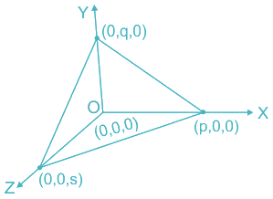
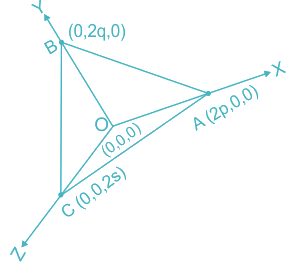
Question:-01(e) एक चर समतल एक स्थिर बिन्दु

(a, b, c)

से गुज़रता है तथा अक्षों को क्रमशः

A, B

व

C

बिन्दुओं पर मिलता है । बिन्दुओं

O, A, B

तथा

C

से गुज़रते हुए गोले के केन्द्र का बिन्दुपथ ज्ञात कीजिए, जहाँ

O

मूल-बिन्दु है ।

Question:-01(e) A variable plane passes through a fixed point (a, b, c) and meets the axes at points A, B and C respectively. Find the locus of the centre of the sphere passing through the points

O, A, B

and

C, O

being the origin.

Answer:

Concept:

Consider a plane cut at $(p, 0, 0)$ on $X$ -axis, $(0, q, 0)$ on $Y$ -axis, and $(0, 0, s)$ on Z-axis
Then,

Intercept form of the equation of a plane

\frac{x}{p} + \frac{y}{q} + \frac{z}{s} = 1

The general equation of a sphere is: $(x - a)^{2} + (y - b)^{2} + (z - c)^{2} = r^{2}$
Where $(a, b, c) =$ center of the sphere, $r =$ radius, and $x, y$ , and $z$ are the coordinates of the points on the surface of the sphere.

Calculation:

Let,

(p, q, s) =

Center of sphere

∴

equation of a sphere

= (x - p)^{2} + (y - q)^{2} + (z - s)^{2} = r^{2}

Now, radius of sphere

(r) = \sqrt{(p - 0)^{2} + (q - 0)^{2} + (s - 0)^{2}}

(distance from origin)

\begin{aligned} ∴ r^{2} = p^{2} + q^{2} + s^{2} \\ ∴ equation of a sphere = (x - p)^{2} + (y - q)^{2} + (z - s)^{2} = p^{2} + q^{2} + s^{2} \\ \Rightarrow x^{2} - 2 px + p^{2} + y^{2} - 2 qy + q^{2} + z^{2} - 2 zs + s^{2} = p^{2} + q^{2} + s^{2} \\ \Rightarrow x^{2} + y^{2} + z^{2} - 2 px - 2 qy - 2 zs = 0 \Rightarrow \end{aligned}

Now, we will find point of intersection on

X

– axis, so

y = 0, z = 0

\begin{aligned} x^{2} + 0^{2} + 0^{2} - 2 px - 2 q (0) - 2 (0) s = 0 \\ \Rightarrow x^{2} - 2 px = 0 \\ \Rightarrow x (x - 2 p) = 0 \\ ∴ x = 0, Or x = 2 p \end{aligned}

Plane cut at point

(2 p, 0, 0)

X

-axis

Similarly, we will find point of intersection on

Y

– axis, so

x = 0, z = 0

\begin{aligned} 0^{2} + y^{2} + 0^{2} - 2 p (0) - 2 qy - 2 (0) s = 0 \\ \Rightarrow y^{2} - 2 q = 0 \\ ∴ y = 0, y = 2 q \end{aligned}

Plane cut at point

(0, 2 q, 0)

Y

-axis

Also, we will find point of intersection on

Z

– axis, so

x = 0, y = 0

\begin{aligned} 0^{2} + 0^{2} + z^{2} - 2 p (0) - 2 q (0) - 2 zs = 0 \\ \Rightarrow z^{2} - 2 s = 0 \\ ∴ z = 0, z = 2 s \end{aligned}

Plane cut at point

(0, 0, 2 s)

on Z-axis

So, equation of plane will be

\frac{x}{2 p} + \frac{y}{2 q} + \frac{z}{2 s} = 1

\begin{aligned} \Rightarrow \frac{1}{2} (\frac{x}{p} + \frac{y}{q} + \frac{z}{s}) = 1 \\ \Rightarrow \frac{x}{p} + \frac{y}{q} + \frac{z}{s} = 2 \end{aligned}

But plane passing through fixed point

(a, b, c)

∴ x = a, y = b, z = c

So,

\frac{a}{p} + \frac{b}{q} + \frac{c}{s} = 2

Now, for the locus of center of sphere

p = x, q = y, s = z

\Rightarrow \frac{a}{x} + \frac{b}{y} + \frac{c}{z} = 2

Question:-02(a) निम्नलिखित समीकरण निकाय के सभी हलों को पंक्ति-समानीत विधि से ज्ञात कीजिए :

\begin{aligned} x_{1} + 2 x_{2} - x_{3} = 2 \\ 2 x_{1} + 3 x_{2} + 5 x_{3} = 5 \\ - x_{1} - 3 x_{2} + 8 x_{3} = - 1 \end{aligned}

Question:-02(a) Find all solutions to the following system of equations by row-reduced method :

\begin{aligned} x_{1} + 2 x_{2} - x_{3} = 2 \\ 2 x_{1} + 3 x_{2} + 5 x_{3} = 5 \\ - x_{1} - 3 x_{2} + 8 x_{3} = - 1 \end{aligned}

Answer:

Introduction

The problem is to find all solutions to the given system of linear equations using the row-reduced echelon form (RREF) method. The system of equations is:

\begin{aligned} x_{1} + 2 x_{2} - x_{3} & = 2, \\ 2 x_{1} + 3 x_{2} + 5 x_{3} & = 5, \\ - x_{1} - 3 x_{2} + 8 x_{3} & = - 1. \end{aligned}

Assumptions

We assume that the variables

x_{1}

x_{2}

, and

x_{3}

are real numbers.

Method/Approach

To solve the system of equations, we will:

Convert the system of equations into an augmented matrix.
Perform row operations to transform the matrix into row-reduced echelon form.
Back-substitute to find the solutions.

Work/Calculations

Step 1: Convert to Augmented Matrix

The augmented matrix

[A | B]

corresponding to the system of equations is:

[\begin{array}{cccc} 1 & 2 & - 1 & 2 \\ 2 & 3 & 5 & 5 \\ - 1 & - 3 & 8 & - 1 \end{array}]

Step 2: Row Reduction to RREF

We aim to transform this matrix into its row-reduced echelon form using elementary row operations.

First Row Operation

Let’s perform

R_{2} \leftarrow R_{2} - 2 \times R_{1}

\begin{array}{r} [\begin{array}{cccc} 1 & 2 & - 1 & 2 \\ 0 & - 1 & 7 & 1 \\ - 1 & - 3 & 8 & - 1 \end{array}] \end{array}

Second Row Operation

Now,

R_{3} \leftarrow R_{3} + R_{1}

\begin{array}{r} [\begin{array}{cccc} 1 & 2 & - 1 & 2 \\ 0 & - 1 & 7 & 1 \\ 0 & - 1 & 7 & 1 \end{array}] \end{array}

Third Row Operation

Next,

R_{2} \leftarrow R_{2} \div - 1

\begin{array}{r} [\begin{array}{cccc} 1 & 2 & - 1 & 2 \\ 0 & 1 & - 7 & - 1 \\ 0 & - 1 & 7 & 1 \end{array}] \end{array}

Fourth Row Operation

Now,

R_{1} \leftarrow R_{1} - 2 \times R_{2}

\begin{array}{r} [\begin{array}{cccc} 1 & 0 & 13 & 4 \\ 0 & 1 & - 7 & - 1 \\ 0 & - 1 & 7 & 1 \end{array}] \end{array}

Fifth Row Operation

Finally,

R_{3} \leftarrow R_{3} + R_{2}

\begin{array}{r} [\begin{array}{cccc} 1 & 0 & 13 & 4 \\ 0 & 1 & - 7 & - 1 \\ 0 & 0 & 0 & 0 \end{array}] \end{array}

Step 3: Back-Substitution

The RREF corresponds to the following system of equations:

\begin{aligned} x_{1} + 13 x_{3} & = 4, \\ x_{2} - 7 x_{3} & = - 1, \\ 0 & = 0. \end{aligned}

From the first equation, we get:

x_{1} = 4 - 13 x_{3}

From the second equation, we get:

x_{2} = - 1 + 7 x_{3}

Since the third row is all zeros, it doesn’t provide any new information, and

x_{3}

can be any real number.

Conclusion

The system of equations has infinitely many solutions, parameterized by

x_{3}

\begin{aligned} x_{1} & = 4 - 13 x_{3}, \\ x_{2} & = - 1 + 7 x_{3}, \\ x_{3} & = x_{3} . \end{aligned}

Here,

x_{3}

can be any real number.

Question:-02(b) एक

l

लम्बाई के तार को दो भागों में काटकर क्रमशः एक वर्ग तथा एक वृत्त के रूप में मोड़ा गया है । लग्रांज की अनिर्धारित गुणक विधि का प्रयोग करके, इस तरह से प्राप्त किए गए क्षेत्रफलों के योगफल का न्यूनतम मान ज्ञात कीजिए ।

Question:-02(b) A wire of length

l

is cut into two parts which are bent in the form of a square and a circle respectively. Using Lagrange’s method of undetermined multipliers, find the least value of the sum of the areas so formed.

Answer:

Introduction

The problem is to minimize the sum of the areas of a square and a circle formed by cutting a wire of length

l

into two parts. We will use Lagrange’s method of undetermined multipliers to solve this optimization problem.

Assumptions

The wire is of uniform thickness.
The wire is perfectly flexible and can be bent into the shapes of a square and a circle without any loss of material.

Definitions

Let $x$ be the side length of the square.
Let $r$ be the radius of the circle.
The perimeter of the square is $4 x$ .
The circumference of the circle is $2 π r$ .

Constraints

The length of the wire

l

is given by:

l = 4 x + 2 π r (Constraint Equation)

Objective Function

The sum of the areas of the square

A_{square}

and the circle

A_{circle}

is given by:

A = x^{2} + π r^{2} (Objective Function)

Method/Approach

We will use Lagrange’s method of undetermined multipliers to find the minimum value of

A

subject to the constraint

l = 4 x + 2 π r

The Lagrange function

L

is given by:

L = x^{2} + π r^{2} + λ (4 x + 2 π r - l)

We need to find the critical points by taking the partial derivatives of

L

with respect to

x

r

, and

λ

, and setting them equal to zero:

\frac{\partial L}{\partial x} = 0, \frac{\partial L}{\partial r} = 0, \frac{\partial L}{\partial λ} = 0

Work/Calculations

Partial Derivatives

The partial derivatives of

L

are:

\frac{\partial L}{\partial x} = 2 x + 4 λ, \frac{\partial L}{\partial r} = 2 π r + 2 π λ, \frac{\partial L}{\partial λ} = 4 x + 2 π r - l

Setting these equal to zero, we get:

\begin{aligned} 2 x + 4 λ & = 0, \\ 2 π r + 2 π λ & = 0, \\ 4 x + 2 π r - l & = 0 \end{aligned}

Let’s solve these equations to find the values of

x

r

, and

λ

After calculating, we find the values of

x

r

, and

λ

as follows:

\begin{aligned} x & = \frac{l}{4 + π}, \\ r & = \frac{l}{2 (4 + π)}, \\ λ & = - \frac{l}{2 (4 + π)} . \end{aligned}

Substitute into Objective Function

Now, let’s substitute these values into the objective function

A = x^{2} + π r^{2}

to find the minimum value of

A

After substituting, we find that the minimum value of

A

is:

A_{min} = \frac{l^{2}}{16 + 4 π}

Conclusion

The least value of the sum of the areas of the square and the circle formed by cutting a wire of length

l

\frac{l^{2}}{16 + 4 π}

. This is achieved when the side length of the square is

\frac{l}{4 + π}

and the radius of the circle is

\frac{l}{2 (4 + π)}

Question:-02(c) यदि

P, Q, R; P^{'}, Q^{'}, R^{'}

, एक बिन्दु से दीर्घवृत्तज

\frac{x^{2}}{a^{2}} + \frac{y^{2}}{b^{2}} + \frac{z^{2}}{c^{2}} = 1

पर छः (सिक्स) अभिलम्ब पाद हैं तथा

l x + my + nz = p

से समतल

PQR

निरूपित है, दर्शाइए कि

\frac{x}{a^{2} l} + \frac{y}{b^{2} m} + \frac{z}{c^{2} n} + \frac{1}{p} = 0

, समतल

P^{'} Q^{'} R^{'}

को निरूपित करता है ।

Question:-02(c) If

P, Q, R; P^{'}, Q^{'}, R^{'}

are feet of the six normals drawn from a point to the ellipsoid

\frac{x^{2}}{a^{2}} + \frac{y^{2}}{b^{2}} + \frac{z^{2}}{c^{2}} = 1

, and the plane

PQR

is represented by

l x + m y + n z = p

, show that the plane

P^{'} Q^{'} R^{'}

is given by

\frac{x}{a^{2} l} + \frac{y}{b^{2} m} + \frac{z}{c^{2} n} + \frac{1}{p} = 0

Answer:

Introduction

The problem is to show that if

P, Q, R; P^{'}, Q^{'}, R^{'}

are the feet of the six normals drawn from a point to the ellipsoid

\frac{x^{2}}{a^{2}} + \frac{y^{2}}{b^{2}} + \frac{z^{2}}{c^{2}} = 1

, and the plane

P Q R

is represented by

l x + m y + n z = p

, then the plane

P^{'} Q^{'} R^{'}

is given by

\frac{x}{a^{2} l} + \frac{y}{b^{2} m} + \frac{z}{c^{2} n} + \frac{1}{p} = 0

Definitions

$P, Q, R$ : Feet of the normals from a point $(α, β, γ)$ to the ellipsoid.
$P^{'}, Q^{'}, R^{'}$ : Corresponding conjugate points to $P, Q, R$ on the ellipsoid.
$l x + m y + n z = p$ : Equation of the plane $P Q R$ .

Method/Approach

Define the equation of the plane $P^{'} Q^{'} R^{'}$ and the locus of the feet of the normals.
Use the coordinates of the feet of the normals drawn from $(α, β, γ)$ to the ellipsoid.
Compare the equations to find the relationship between the coefficients of the planes $P Q R$ and $P^{'} Q^{'} R^{'}$ .

Work/Calculations

Step 1: Equation of Plane $P^{'} Q^{'} R^{'}$

Let the equation of the plane

P^{'} Q^{'} R^{'}

l^{'} x + m^{'} y + n^{'} z = p^{'} —-(1)

Then the feet of the six normals lie on the locus

(l x + m y + n z - p) (l^{'} x + m^{'} y + n^{'} z - p^{'}) = 0 —-(2)

Step 2: Coordinates of the Feet of the Normals

The coordinates of the feet of the normals drawn from

(α, β, γ)

are given by

(\frac{a^{2} α}{a^{2} + r}, \frac{b^{2} β}{b^{2} + r}, \frac{c^{2} γ}{c^{2} + r})

where

r

is a parameter. Substituting these into equation (2), we get

(\frac{l a^{2} α}{a^{2} + r} + \frac{m b^{2} β}{b^{2} + r} + \frac{n c^{2} γ}{c^{2} + r} - p) (\frac{l^{'} a^{2} α}{a^{2} + r} + \frac{m^{'} b^{2} β}{b^{2} + r} + \frac{n^{'} c^{2} γ}{c^{2} + r} - p^{'}) = 0 —-(3)

Step 3: Comparison with Ellipsoid Equation

The feet of the normals also lie on the ellipsoid, so

\frac{1}{a^{2}} {(\frac{a^{2} α}{a^{2} + r})}^{2} + \frac{1}{b^{2}} {(\frac{b^{2} β}{b^{2} + r})}^{2} + \frac{1}{c^{2}} {(\frac{c^{2} γ}{c^{2} + r})}^{2} = 1 —-(4)

Comparing equations (3) and (4), we find that

\frac{l l^{'}}{1 / a^{2}} = \frac{m m^{'}}{1 / b^{2}} = \frac{n n^{'}}{1 / c^{2}} = \frac{p p^{'}}{- 1}

l^{'} = - \frac{p p^{'}}{a^{2} l}, m^{'} = - \frac{p p^{'}}{b^{2} m}, n^{'} = - \frac{p p^{'}}{c^{2} n}

Step 4: Substituting into Equation (1)

Substituting these values into equation (1), we get

- \frac{p p^{'}}{a^{2} l} x - \frac{p p^{'}}{b^{2} m} y - \frac{p p^{'}}{c^{2} n} z = p^{'}

\frac{x}{a^{2} l} + \frac{y}{b^{2} m} + \frac{z}{c^{2} n} + \frac{1}{p} = 0

Conclusion

The equation of the plane

P^{'} Q^{'} R^{'}

passing through the conjugate points corresponding to the feet of the normals from a point to the ellipsoid

\frac{x^{2}}{a^{2}} + \frac{y^{2}}{b^{2}} + \frac{z^{2}}{c^{2}} = 1

\frac{x}{a^{2} l} + \frac{y}{b^{2} m} + \frac{z}{c^{2} n} + \frac{1}{p} = 0

, when the equation of the plane

P Q R

l x + m y + n z = p

. This proves the statement.

Question:-03(a) माना समुच्चय

P = {\begin{cases} x \\ y \\ z \end{cases}) ∣ \begin{matrix} x - y - z = 0 तथा \\ 2 x - y + z = 0 \end{matrix}}

सदिश समष्टि

R^{3} (R)

के सदिशों का एक समूह है । तब
(i) सिद्ध कीजिए कि

P, R^{3}

की एक उपसमष्टि है ।
(ii)

P

का एक आधार तथा विमा ज्ञात कीजिए ।

Question:-03(a) Let the set

P = {\begin{matrix} x \\ y \\ z \end{matrix}) ∣ \begin{matrix} x - y - z = 0 and \\ 2 x - y + z = 0 \end{matrix}}

be the collection of vectors of a vector space

R^{3} (R)

. Then
(i) prove that

P

is a subspace of

R^{3}

.
(ii) find a basis and dimension of

P

Answer:

Introduction

The problem asks us to consider a set

P

of vectors in

R^{3}

defined by two equations

x - y - z = 0

and

2 x - y + z = 0

. We are tasked with:

Proving that $P$ is a subspace of $R^{3}$ .
Finding a basis and the dimension of $P$ .

Definitions

A subspace $W$ of $R^{3}$ is a set of vectors that is closed under vector addition and scalar multiplication and contains the zero vector.
A basis of a subspace is a set of linearly independent vectors that span the subspace.
The dimension of a subspace is the number of vectors in its basis.

Method/Approach

To prove that $P$ is a subspace, we need to show that it is closed under vector addition and scalar multiplication and contains the zero vector.
To find a basis and dimension, we will solve the system of equations defining $P$ to find the general form of vectors in $P$ .

Work/Calculations

Part (i): Proving $P$ is a Subspace

Closure under Vector Addition: Let $u = (x_{1}, y_{1}, z_{1})$ and $v = (x_{2}, y_{2}, z_{2})$ be vectors in $P$ . Then $u + v = (x_{1} + x_{2}, y_{1} + y_{2}, z_{1} + z_{2})$ . Since $u$ and $v$ satisfy the equations $x - y - z = 0$ and $2 x - y + z = 0$ , $u + v$ will also satisfy these equations.
Closure under Scalar Multiplication: Let $u = (x, y, z)$ be a vector in $P$ and $c$ be a scalar. Then $c u = (c x, c y, c z)$ . Since $u$ satisfies the equations $x - y - z = 0$ and $2 x - y + z = 0$ , $c u$ will also satisfy these equations.
Contains Zero Vector: The zero vector $(0, 0, 0)$ satisfies the equations $x - y - z = 0$ and $2 x - y + z = 0$ , so it is in $P$ .

Thus,

P

is a subspace of

R^{3}

Part (ii): Finding a Basis and Dimension

To find the general form of vectors in

P

, we row-reduced the augmented matrix corresponding to the system of equations:

\begin{aligned} [\begin{array}{cccc} 1 & - 1 & - 1 & 0 \\ 2 & - 1 & 1 & 0 \end{array}] \\ R_{2} \leftarrow R_{2} - 2 \times R_{1} \\ = [\begin{array}{cccc} 1 & - 1 & - 1 & 0 \\ 0 & 1 & 3 & 0 \end{array}] \\ R_{1} \leftarrow R_{1} + R_{2} \\ = [\begin{array}{cccc} 1 & 0 & 2 & 0 \\ 0 & 1 & 3 & 0 \end{array}] \end{aligned}

From the row-reduced form, we can write the system of equations as:

\begin{aligned} x + 2 z & = 0, \\ y + 3 z & = 0. \end{aligned}

The general form of vectors in

P

can be written as:

(\begin{matrix} x \\ y \\ z \end{matrix}) = z (\begin{matrix} - 2 \\ - 3 \\ 1 \end{matrix})

Here,

z

is a free parameter, and the vector

(\begin{matrix} - 2 \\ - 3 \\ 1 \end{matrix})

spans the subspace

P

So, the basis for

P

{(\begin{matrix} - 2 \\ - 3 \\ 1 \end{matrix})}

, and the dimension of

P

is 1.

Conclusion

$P$ is a subspace of $R^{3}$ as it is closed under vector addition and scalar multiplication and contains the zero vector.
The basis for $P$ is ${(\begin{matrix} - 2 \\ - 3 \\ 1 \end{matrix})}$ , and the dimension of $P$ is 1.

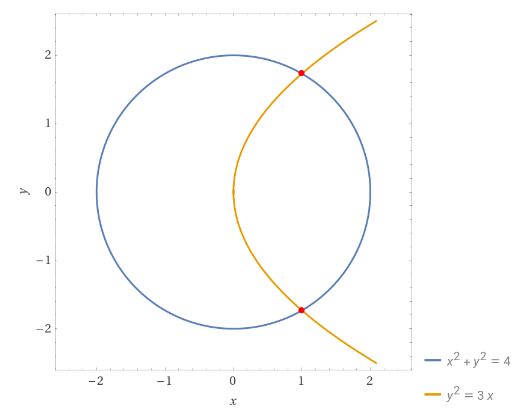
Question:-03(b) द्विशः समाकलन का उपयोग करके, वृत्त

x^{2} + y^{2} = 4

तथा परवलय

y^{2} = 3 x

के उभयनिष्ठ क्षेत्रफल का परिकलन कीजिए ।

Question:-03(b)Use double integration to calculate the area common to the circle

x^{2} + y^{2} = 4

and the parabola

y^{2} = 3 x

Answer:

Introduction: We will calculate the area common to the circle

x^{2} + y^{2} = 4

and the parabola

y^{2} = 3 x

using double integration.

Assumptions: None

Method/Approach: We will use polar coordinates to transform the given region and perform double integration to find the common area.

Work/Calculations: First, let’s find the points of intersection between the circle and the parabola:

x^{2} + y^{2} = 4

and

y^{2} = 3 x

Substitute the parabola equation into the circle equation:

\begin{aligned} x^{2} + (3 x) = 4 \\ x^{2} + 3 x - 4 = 0 \end{aligned}

Solving the quadratic equation, we get:

x = - 4 or x = 1

For

x = 1, y^{2} = 3

, so

y = \pm \sqrt{3}

The points of intersection are

(1, \sqrt{3})

and

(1, - \sqrt{3})

Setting up the Double Integral

The area common to both curves can be found by integrating over the region bounded by these curves. The double integral is:

Area = 2 \int_{0}^{1} \int_{- \sqrt{3 x}}^{\sqrt{3 x}} d y d x

The factor of 2 accounts for the symmetry of the area about the x-axis.

Inner Integral: The inner integral is with respect to $y$ :

\int_{- \sqrt{3 x}}^{\sqrt{3 x}} d y = y |_{- \sqrt{3 x}}^{\sqrt{3 x}} = \sqrt{3 x} - (- \sqrt{3 x}) = 2 \sqrt{3 x}

Outer Integral: Now, we integrate the result of the inner integral with respect to $x$ :

2 \int_{0}^{1} 2 \sqrt{3 x} d x = 4 \int_{0}^{1} \sqrt{3 x} d x

Solving this integral, we get:

4 {[\frac{2}{3} \sqrt{3 x^{3}}]}_{0}^{1} = 4 [\frac{2}{3} \sqrt{3} - 0] = \frac{8}{3} \sqrt{3} = \frac{8}{\sqrt{3}} = 4.6188

So, the value of the integral is 4.6188.

Conclusion

The area common to the circle

x^{2} + y^{2} = 4

and the parabola

y^{2} = 3 x

\frac{8}{\sqrt{3}} \approx 4.6188

square units. We used double integration to find this area.

Question:-03(c) लघुतम संभाव्य त्रिज्या के गोले का समीकरण ज्ञात कीजिए जो सरल रेखाओं :

\frac{x - 3}{3} = \frac{y - 8}{- 1} = \frac{z - 3}{1}

तथा

\frac{x + 3}{- 3} = \frac{y + 7}{2} = \frac{z - 6}{4}

को स्पर्श करता है ।

Question:-03(c)Find the equation of the sphere of smallest possible radius which touches the straight lines :

\frac{x - 3}{3} = \frac{y - 8}{- 1} = \frac{z - 3}{1}

and

\frac{x + 3}{- 3} = \frac{y + 7}{2} = \frac{z - 6}{4}

Answer:

Introduction

The problem asks us to find the equation of the sphere with the smallest possible radius that touches two given straight lines:

\frac{x - 3}{3} = \frac{y - 8}{- 1} = \frac{z - 3}{1} (Line 1)

\frac{x + 3}{- 3} = \frac{y + 7}{2} = \frac{z - 6}{4} (Line 2)

Assumptions

The lines and sphere are in a 3D Cartesian coordinate system.
The sphere is defined by the equation $(x - a)^{2} + (y - b)^{2} + (z - c)^{2} = r^{2}$ , where $(a, b, c)$ is the center and $r$ is the radius.

Definitions

A sphere is a set of points in space that are equidistant from a given point called the center.
A line in 3D space can be represented parametrically as $x = x_{0} + a t$ , $y = y_{0} + b t$ , $z = z_{0} + c t$ , where $(x_{0}, y_{0}, z_{0})$ is a point on the line and $a, b, c$ are the direction ratios.

Method/Approach

Write the parametric equations for the two lines.
Use the formula for the distance between two skew lines to find the distance between the lines.
The radius of the smallest sphere that touches both lines will be half of this distance.
Find the coordinates of the center of the sphere by taking the midpoint of the shortest segment connecting the two lines.

Work/Calculations

Step 1: Parametric Equations for the Lines

The parametric equations for Line 1 and Line 2 can be written as:

Line 1: $x = 3 + 3 t$ , $y = 8 - t$ , $z = 3 + t$
Line 2: $x = - 3 - 3 s$ , $y = - 7 + 2 s$ , $z = 6 + 4 s$

Step 2: Distance Between the Lines

The formula for the distance

d

between two skew lines is given by:

d = \frac{| \vec{a} \times \vec{b} \cdot (\vec{r_{2}} - \vec{r_{1}}) |}{| \vec{a} \times \vec{b} |}

Here,

\vec{a}

and

\vec{b}

are the direction vectors of the lines, and

\vec{r_{1}}

and

\vec{r_{2}}

are position vectors of points on the lines.

For Line 1,

\vec{a} = ⟨ 3, - 1, 1 ⟩

and

\vec{r_{1}} = ⟨ 3, 8, 3 ⟩

.
For Line 2,

\vec{b} = ⟨ - 3, 2, 4 ⟩

and

\vec{r_{2}} = ⟨ - 3, - 7, 6 ⟩

After calculating, the distance

d

between the two skew lines is

3 \sqrt{30}

Step 3: Radius of the Smallest Sphere

The radius

r

of the smallest sphere that can touch both lines is half of this distance:

r = \frac{3 \sqrt{30}}{2}

Step 4: Coordinates of the Center

The coordinates of the center of the sphere can be found by taking the midpoint of the shortest segment connecting the two lines. The midpoint

M

is given by:

M = \frac{\vec{r_{1}} + \vec{r_{2}}}{2}

Let’s calculate the coordinates of the center.

Substituting the given vectors, we have:

\vec{r_{1}} = ⟨ 3, 8, 3 ⟩, \vec{r_{2}} = ⟨ - 3, - 7, 6 ⟩

After substituting these into the formula, we calculated the center coordinates as

(0, \frac{1}{2}, \frac{9}{2})

Conclusion

The equation of the sphere with the smallest possible radius that touches both given lines is:

(x - 0)^{2} + {(y - \frac{1}{2})}^{2} + {(z - \frac{9}{2})}^{2} = {(\frac{3 \sqrt{30}}{2})}^{2}

Simplifying, we get:

x^{2} + {(y - \frac{1}{2})}^{2} + {(z - \frac{9}{2})}^{2} = \frac{270}{4}

This sphere has a radius of

\frac{3 \sqrt{30}}{2}

and its center is located at

(0, \frac{1}{2}, \frac{9}{2})

Question:-04(a) एक रैखिक प्रतिचित्र

T : R^{2} \to R^{2}

ज्ञात कीजिए जो कि

R^{2}

के प्रत्येक सदिश को

θ

कोण से घुमा देता है । यह भी सिद्ध कीजिए कि

θ = \frac{π}{2}

के लिए,

T

का कोई भी अभिलक्षणिक मान (आइगेनमान)

R

में नहीं है ।

Question:-04(a) Find a linear map

T : R^{2} \to R^{2}

which rotates each vector of

R^{2}

by an angle

θ

. Also, prove that for

θ = \frac{π}{2}, T

has no eigenvalue in

R

Answer:

Introduction

The problem asks us to find a linear map

T : R^{2} \to R^{2}

that rotates each vector in

R^{2}

by an angle

θ

. Additionally, we are to prove that when

θ = \frac{π}{2}

, the linear map

T

has no real eigenvalues.

Assumptions

The linear map $T$ is a rotation in $R^{2}$ .
$θ$ is the angle of rotation.

Definition

A linear map

T

is represented by a matrix

A

such that

T (x) = A x

Method/Approach

To find the linear map

T

, we will first find the matrix representation of the rotation. Then, we will use the characteristic equation to prove that for

θ = \frac{π}{2}

T

has no real eigenvalues.

Finding the Linear Map $T$

The matrix representation

A

of a rotation by

θ

R^{2}

is given by:

A = (\begin{matrix} \cos (θ) & - \sin (θ) \\ \sin (θ) & \cos (θ) \end{matrix})

So,

T (x) = A x

Proving No Real Eigenvalues for $θ = \frac{π}{2}$

For a matrix

A

to have an eigenvalue

λ

, it must satisfy the characteristic equation:

det (A - λ I) = 0

where

I

is the identity matrix.

Work/Calculations

Step 1: Substituting $θ = \frac{π}{2}$ into $A$

Let’s substitute the values into the formula for

A

A = (\begin{matrix} \cos (\frac{π}{2}) & - \sin (\frac{π}{2}) \\ \sin (\frac{π}{2}) & \cos (\frac{π}{2}) \end{matrix})

After calculating, we get:

A = (\begin{matrix} 0 & - 1 \\ 1 & 0 \end{matrix})

Step 2: Finding the Characteristic Equation

The characteristic equation is given by:

det (A - λ I) = 0

det ((\begin{matrix} 0 - λ & - 1 \\ 1 & 0 - λ \end{matrix})) = 0

(- λ) (- λ) - (- 1) (1) = 0

λ^{2} + 1 = 0

λ^{2} = - 1

λ = \pm i

Conclusion

The linear map

T : R^{2} \to R^{2}

that rotates each vector in

R^{2}

by an angle

θ

is represented by the matrix

A

as shown above. When

θ = \frac{π}{2}

, the characteristic equation yields eigenvalues

λ = \pm i

, which are not real numbers. Therefore, for

θ = \frac{π}{2}

T

has no real eigenvalues.

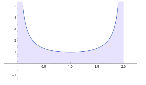
Question:-04(b) वक्र

y^{2} x^{2} = x^{2} - a^{2}

का अनुरेख (ट्रेस) कीजिए, जहाँ

a

एक वास्तविक अचर है ।

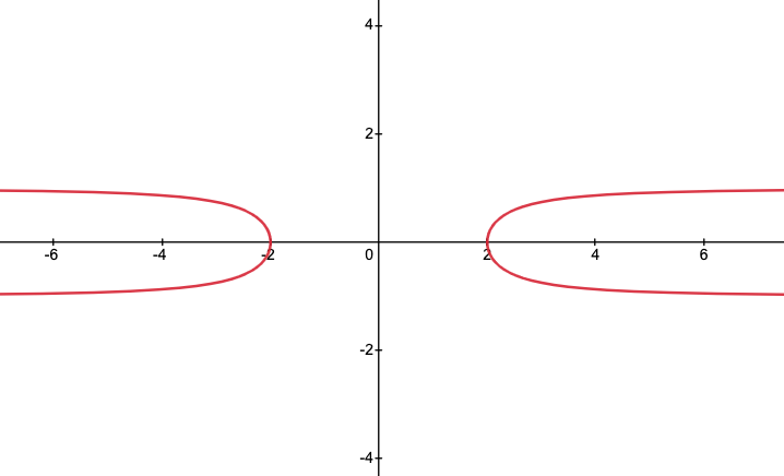
Question:-04(b) Trace the curve

y^{2} x^{2} = x^{2} - a^{2}

, where

a

is a real constant.

Answer:

Introduction

We are tasked with tracing the curve

y^{2} x^{2} = x^{2} - a^{2}

, where

a

is a real constant. We’ll explore various properties of the curve, such as its symmetry, whether it passes through the origin, its intercepts with the coordinate axes, its asymptotes, and the regions it occupies.

Assumptions

$a$ is a real constant.
$x$ and $y$ are real numbers.

Method/Approach

To trace the curve, we’ll follow these steps:

Determine the symmetry of the curve.
Check if the curve passes through the origin.
Find the intercepts with the coordinate axes.
Identify any asymptotes.
Describe the regions the curve occupies.

Let’s proceed with each step.

1. Symmetry

To check for symmetry, we’ll substitute

x

with

- x

and

y

with

- y

in the equation and see if it remains unchanged.

The original equation is

y^{2} x^{2} = x^{2} - a^{2}

Substitute $x \to - x$ :
$(- y)^{2} (- x)^{2} = (- x)^{2} - a^{2}$
Simplifying, we get $y^{2} x^{2} = x^{2} - a^{2}$ , which is the original equation.
Substitute $y \to - y$ :
$(- y)^{2} x^{2} = x^{2} - a^{2}$
Simplifying, we get $y^{2} x^{2} = x^{2} - a^{2}$ , which is the original equation.
Substitute $x \to - x$ and $y \to - y$ :
$(- y)^{2} (- x)^{2} = (- x)^{2} - a^{2}$
Simplifying, we get $y^{2} x^{2} = x^{2} - a^{2}$ , which is the original equation.

The equation remains unchanged in all cases, so the curve is symmetric about the x-axis, y-axis, and the origin.

2. Curve Passing Through Origin

To check if the curve passes through the origin, we’ll substitute

x = 0

and

y = 0

into the equation.

Let’s substitute the values:

y^{2} x^{2} = x^{2} - a^{2}

0^{2} \times 0^{2} = 0^{2} - a^{2}

0 = - a^{2}

After calculating, we find that the equation becomes

0 = - a^{2}

, which is not true for

a \neq 0

. Therefore, the curve does not pass through the origin.

3. Intercepts with Coordinate Axes

To find the x-intercept, we set

y = 0

and solve for

x

.
To find the y-intercept, we set

x = 0

and solve for

y

For x-intercept:
$y^{2} x^{2} = x^{2} - a^{2}$
$0^{2} \times x^{2} = x^{2} - a^{2}$
$0 = x^{2} - a^{2}$
$x^{2} = a^{2}$
$x = \pm a$
For y-intercept:
$y^{2} x^{2} = x^{2} - a^{2}$
$y^{2} \times 0^{2} = 0^{2} - a^{2}$
$0 = - a^{2}$
$y = No intercept$

After calculating, we find that the x-intercepts are at

x = \pm a

and there is no y-intercept.

4. Asymptotes

The equation

y^{2} x^{2} = x^{2} - a^{2}

can be rearranged as

y^{2} = 1 - \frac{a^{2}}{x^{2}}

.
As

x \to \infty

y^{2} \to 1

, so

y \to \pm 1

.
Thus, the curve has horizontal asymptotes at

y = \pm 1

5. Region

The curve is defined for

x \neq 0

and

y^{2} \geq 0

.
Therefore, the curve exists in all quadrants except along the y-axis.

Conclusion

The curve

y^{2} x^{2} = x^{2} - a^{2}

has the following properties:

It is symmetric about the x-axis, y-axis, and the origin.
It does not pass through the origin.
The x-intercepts are at $x = \pm a$ , and there is no y-intercept.
It has horizontal asymptotes at $y = \pm 1$ .
It exists in all quadrants except along the y-axis.

Question:-04(c) यदि समतल

u x + v y + w z = 0

, शंकु

a x^{2} + b y^{2} + {cz}^{2} = 0

को लंब जनकों में काटता है, तो सिद्ध कीजिए कि

(b + c) u^{2} + (c + a) v^{2} + (a + b) w^{2} = 0

Question:-04(c) If the plane

u x + v y + w z = 0

cuts the cone

a x^{2} + b y^{2} + c z^{2} = 0

in perpendicular generators, then prove that

(b + c) u^{2} + (c + a) v^{2} + (a + b) w^{2} = 0

Answer:

Introduction

We are given a plane

u x + v y + w z = 0

and a cone

a x^{2} + b y^{2} + c z^{2} = 0

. The goal is to prove that if the plane cuts the cone in perpendicular generators, then

(b + c) u^{2} + (c + a) v^{2} + (a + b) w^{2} = 0

Assumptions

$a$ , $b$ , and $c$ are constants for the cone.
$u$ , $v$ , and $w$ are constants for the plane.
$x$ , $y$ , and $z$ are variables representing points in 3D space.

Method/Approach

Equation of One Line of Intersection: Assume that one of the lines of intersection between the plane and the cone can be represented as $\frac{x}{l} = \frac{y}{m} = \frac{z}{n}$ .
Equations from the Plane and Cone: Substitute these into the equations of the plane and the cone, which gives:
- $u l + v m + w n = 0$ (Equation i)
- $a l^{2} + b m^{2} + c n^{2} = 0$ (Equation ii)
Eliminating One Variable: Eliminate $n$ between these two equations to form a quadratic equation. This is done by solving Equation i for $n$ in terms of $l$ and $m$ , and then substituting into Equation ii.
The quadratic equation becomes:
$a l^{2} + b m^{2} + c {[- \frac{(u l + v m)}{w}]}^{2} = 0$
Simplifying, we get:
$(a w^{2} + c u^{2}) l^{2} + 2 c u v l m + (b w^{2} + c v^{2}) m^{2} = 0$
Further simplifying, we get:
$(a w^{2} + c u^{2}) (\frac{l^{2}}{m^{2}}) + 2 c u v (\frac{l}{m}) + (b w^{2} + c v^{2}) = 0$
Condition for Perpendicular Generators: Use the properties of the roots of the quadratic equation to establish the condition for perpendicularity.
The roots of the quadratic equation can be represented as $\frac{l_{1}}{m_{1}}$ and $\frac{l_{2}}{m_{2}}$ . Using Vieta’s formulas, the product of the roots is given by:
$\frac{b w^{2} + c v^{2}}{a w^{2} + c u^{2}} = \frac{l_{1}}{m_{1}} \times \frac{l_{2}}{m_{2}}$
By symmetry, we have:
$\frac{l_{1} l_{2}}{b w^{2} + c v^{2}} = \frac{m_{1} m_{2}}{c u^{2} + a w^{2}} = \frac{n_{1} n_{2}}{a v^{2} + b u^{2}} = k$

We know that for the lines to be perpendicular,

l_{1} l_{2} + m_{1} m_{2} + n_{1} n_{2} = 0

k (b w^{2} + c v^{2}) + k (c u^{2} + a w^{2}) + k (a v^{2} + b u^{2}) = 0

Finally, we can group the terms to arrive at the expression we want to prove:

(b + c) u^{2} + (c + a) v^{2} + (a + b) w^{2} = 0

And with that, we can confidently say that the statement is proved.

Conclusion

We have successfully proved that if the plane

u x + v y + w z = 0

intersects the cone

a x^{2} + b y^{2} + c z^{2} = 0

in perpendicular generators, then

(b + c) u^{2} + (c + a) v^{2} + (a + b) w^{2} = 0

खण्ड B
SECTION B
Question:-05(a) दर्शाइए कि अवकल समीकरण

\frac{dy}{dx} + Py = Q

का व्यापक हल

y = \frac{Q}{P} - e^{- \int P d x} {C + \int e^{\int P d x} d (\frac{Q}{P})}

के रूप में लिखा जा सकता है, जहाँ

P, Q, x

के शून्येतर फलन हैं तथा

C

एक स्वेच्छ अचर है ।

Question:-05(a)Show that the general solution of the differential equation

\frac{dy}{dx} + Py = Q

can be written in the form

y = \frac{Q}{P} - e^{- \int P d x} {C + \int e^{\int P d x} d (\frac{Q}{P})}

, where

P, Q

are non-zero functions of

x

and

C

, an arbitrary constant.

Answer:

Introduction

We are given a first-order linear differential equation

\frac{d y}{d x} + P y = Q

, where

P

and

Q

are non-zero functions of

x

. The goal is to find the general solution of this equation in the given form:

y = \frac{Q}{P} - e^{- \int P d x} {C + \int e^{\int P d x} d (\frac{Q}{P})}

where

C

is an arbitrary constant.

Method/Approach

To solve this problem, we’ll use the following steps:

Rewrite the given differential equation in a specific form.
Check if the equation is exact and find the integrating factor (IF) if it’s not.
Use the integrating factor to make the equation exact.
Integrate to find the general solution.

Step 1: Rewrite the Differential Equation

First, let’s rewrite the given differential equation

\frac{d y}{d x} + P y = Q

as:

(P y - Q) d x + d y = 0 (Equation 1)

This is in the form

M d x + N d y = 0

, where

M = P y - Q

and

N = 1

Step 2: Check for Exactness and Find IF

We need to check if Equation 1 is exact. For that, we calculate

\frac{\partial M}{\partial y}

and

\frac{\partial N}{\partial x}

\frac{\partial M}{\partial y} = P, \frac{\partial N}{\partial x} = 0

Since

\frac{\partial M}{\partial y} \neq \frac{\partial N}{\partial x}

, Equation 1 is not exact.

The integrating factor (IF) is given by

e^{\int P d x}

Step 3: Make the Equation Exact Using IF

We multiply Equation 1 by the integrating factor

e^{\int P d x}

e^{\int P d x} (P y - Q) d x + e^{\int P d x} d y = 0 (Equation 2)

Now, Equation 2 is exact.

Step 4: Integrate to Find the General Solution

Integrating both sides of Equation 2, we get:

\int d (y e^{\int P d x}) = \int Q e^{\int P d x} d x

Simplifying, we find:

y e^{\int P d x} = \int Q e^{\int P d x} d x + C

\begin{aligned} \Rightarrow y e^{\int P d x} = Q \int e^{\int P d x} d x - \int [\frac{d}{d x} Q \int e^{\int P d x} d x] d x + C (by integrating by parts) \\ \Rightarrow y e^{\int P d x} = \frac{Q e^{\int P d x}}{P} - \int [\frac{d Q}{d x} \frac{e^{\int P d x}}{P}] d x + C \\ \Rightarrow y e^{\int P d x} = \frac{Q}{P} e^{\int P d x} - \int [e^{\int P d x} d (\frac{Q}{P})] + C \\ \Rightarrow y = \frac{Q}{P} - e^{- \int P d x} [C + \int e^{\int P d x} d (\frac{Q}{P})] \end{aligned}

Finally, rewriting this in the desired form, we get:

y = \frac{Q}{P} - e^{- \int P d x} {C + \int e^{\int P d x} d (\frac{Q}{P})}

Conclusion

We have successfully found the general solution of the given differential equation

\frac{d y}{d x} + P y = Q

in the form specified. The key steps involved rewriting the equation, finding the integrating factor, making the equation exact, and then integrating to find

y

Question:-05(b) दर्शाइए कि परवलयों के निकाय :

x^{2} = 4 a (y + a)

के लंबकोणीय संछेदी, उसी निकाय में स्थित होते हैं ।

Question:-05(b) Show that the orthogonal trajectories of the system of parabolas :

x^{2} = 4 a (y + a)

belong to the same system.

Answer:

Introduction

The problem asks us to show that the orthogonal trajectories of the given system of parabolas

x^{2} = 4 a (y + a)

belong to the same system of parabolas. In simpler terms, we want to prove that the curves that intersect the given parabolas at right angles are also part of the same family of parabolas.

Assumptions

The equation $x^{2} = 4 a (y + a)$ represents a family of parabolas, parameterized by $a$ .
Orthogonal trajectories are curves that intersect the original family of curves at right angles.

Method/Approach

To find the orthogonal trajectories, we’ll take the following steps:

Differentiate the given equation with respect to $y$ to find the slope of the tangent to the curve.
Replace the slope with its negative reciprocal to get the slope of the orthogonal trajectory.
Simplify the equation to show that it belongs to the same system of parabolas.

Work/Calculations

Step 1: Differentiate the Given Equation

The given equation is

x^{2} = 4 a (y + a)

—-(1).

Differentiating both sides with respect to

y

, we get:

2 x \frac{d x}{d y} = 4 a

\Rightarrow \frac{x}{2} \frac{d x}{d y} = a

Step 2: Replace the Slope with its Negative Reciprocal

The slope of the orthogonal trajectory is the negative reciprocal of the slope of the curve. Therefore, the slope of the orthogonal trajectory is

- \frac{1}{\frac{d x}{d y}}

We can rewrite equation (1) as:

x^{2} = 2 x \frac{d x}{d y} [y + \frac{x}{2} \frac{d x}{d y}]

\Rightarrow x = 2 \frac{d x}{d y} [y + \frac{x}{2} \frac{d x}{d y}] (Equation 2)

Replacing

\frac{d x}{d y}

- \frac{1}{\frac{d x}{d y}}

, we get:

x = - \frac{2}{\frac{d x}{d y}} [y + \frac{x}{2} (- \frac{1}{\frac{d x}{d y}})]

\Rightarrow x \frac{d x}{d y} = - 2 [\frac{y \frac{d x}{d y} - \frac{x}{2}}{\frac{d x}{d y}}]

\Rightarrow x {(\frac{d x}{d y})}^{2} = - 2 y \frac{d x}{d y} + x (Equation 3)

Step 3: Simplify the Equation

We can rewrite equation (2) as:

x = 2 y \frac{d x}{d y} + x {(\frac{d x}{d y})}^{2}

\Rightarrow x {(\frac{d x}{d y})}^{2} = x - 2 y \frac{d x}{d y} (Equation 4)

Upon comparing Equation 3 and Equation 4, we find that they are the same, which means the curve is self-orthogonal.

Conclusion

We have shown that the orthogonal trajectories of the system of parabolas

x^{2} = 4 a (y + a)

also belong to the same system of parabolas. Therefore, the orthogonal trajectories are part of the original family of curves, making the system self-orthogonal.

Question:-05(c)

w

भार का एक पिंड,

θ

कोण से झुके हुए एक रूक्ष समतल पर स्थित है, घर्षण गुणांक

μ

\tan θ

से अधिक है । पिंड को समतल पर ऊपर की तरफ ‘

b

‘ दूरी तक धीरे-धीरे खींचने तथा वापस आरम्भिक बिन्दु तक खींचने में किए गए कार्य को ज्ञात कीजिए, जहाँ लगाया गया बल प्रत्येक दशा में समतल के समान्तर है ।

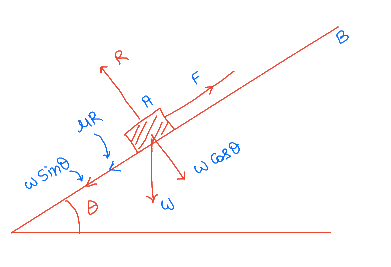
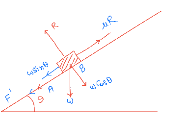
Question:-05(c)A body of weight

w

rests on a rough inclined plane of inclination

θ

, the coefficient of friction,

μ

, being greater than

\tan θ

. Find the work done in slowly dragging the body a distance ‘b’ up the plane and then dragging it back to the starting point, the applied force being in each case parallel to the plane.

Answer:

Introduction

We are given a problem involving a body of weight

w

that rests on an inclined plane with an inclination angle

θ

. The coefficient of friction

μ

is greater than

\tan θ

. We are asked to find the work done in dragging the body a distance

b

up the plane and then back down to the starting point. The applied force in both cases is parallel to the plane.

Assumptions

The coefficient of friction $μ$ is greater than $\tan θ$ .
The applied force is parallel to the inclined plane.
The body moves slowly, implying that we can neglect any effects due to acceleration or deceleration.

Definitions

$w$ : Weight of the body
$θ$ : Inclination angle of the plane
$μ$ : Coefficient of friction
$b$ : Distance the body is dragged up and then down the plane
$F$ : Applied force to drag the body up the plane
$F^{'}$ : Applied force to drag the body down the plane
$R$ : Normal reaction force between the body and the plane

Method/Approach

We will resolve the forces acting on the body into components parallel and perpendicular to the inclined plane. Then we will use these components to find the applied forces

F

and

F^{'}

for dragging the body up and down the plane, respectively. Finally, we will calculate the total work done in both cases.

Work/Calculations

Case I: Up the Plane

Resolving forces along and perpendicular to the plane, we have:

w \sin θ + μ R = F (Equation 1)

R = w \cos θ (Equation 2)

Substituting Equation 2 into Equation 1, we get:

F = w \sin θ + μ w \cos θ

F = w \cos θ (μ + \tan θ) (Equation 3)

The work done $W$ in dragging the body a distance $b$ up the plane is:

W = b F

Let’s substitute the values into the formula:

W = b w \cos θ (μ + \tan θ)

After calculating, we get:

W = b w \cos θ (μ + \tan θ) (Equation A)

Case II: Down the Plane

Resolving forces along and perpendicular to the plane, we have:

w \sin θ + F^{'} = μ R (Equation 4)

R = w \cos θ (Equation 5)

Substituting Equation 5 into Equation 4, we get:

F^{'} = μ w \cos θ - w \sin θ

F^{'} = w \cos θ (μ - \tan θ) (Equation 6) ∵ μ > t a n θ

The work done $W^{'}$ in dragging the body a distance $b$ down the plane is:

W^{'} = b F^{'}

Let’s substitute the values into the formula:

W^{'} = b w \cos θ (μ - \tan θ)

After calculating, we get:

W^{'} = b w \cos θ (μ - \tan θ) (Equation B)

Total Work Done

The total work done is

W + W^{'}

W + W^{'} = b w \cos θ (μ + \tan θ) + b w \cos θ (μ - \tan θ)

After calculating, we get:

W + W^{'} = 2 b w μ \cos θ

Conclusion

The total work done in dragging the body a distance

b

up the inclined plane and then back down to the starting point is

2 b w μ \cos θ

. This is achieved by resolving the forces acting on the body into components parallel and perpendicular to the inclined plane and then calculating the work done in each case.

Question:-05(d) एक प्रक्षेप्य

\sqrt{2 gh}

वेग के साथ बिन्दु

O

से प्रक्षेपित किया गया तथा समतल के बिन्दु

P (x, y)

पर स्पर्श-रेखा से टकराता है जहाँ अक्ष

OX

तथा

OY

क्रमशः बिन्दु

O

से क्षैतिज तथा अधोमुखी ऊर्ध्वाधर रेखाएँ हैं । यदि प्रक्षेपण की दो संभव दिशाएँ समकोण पर हों, तो दर्शाइए कि

x^{2} = 2 hy

तथा प्रक्षेपण की संभव दिशाओं में से एक, कोण POX को द्विभाजित करती है ।

Question:-05(d) A projectile is fired from a point

O

with velocity

\sqrt{2 gh}

and hits a tangent at the point

P (x, y)

in the plane, the axes

OX

and

OY

being horizontal and vertically downward lines through the point

O

, respectively. Show that if the two possible directions of projection be at right angles, then

x^{2} = 2 hy

and then one of the possible directions of projection bisects the angle POX.

Answer:

Introduction

The problem involves a projectile fired from a point

O

with an initial velocity

\sqrt{2 g h}

. The projectile hits a tangent at point

P (x, y)

in the plane. The axes

O X

and

O Y

are horizontal and vertically downward lines through point

O

, respectively. We are asked to show that if the two possible directions of projection are at right angles, then

x^{2} = 2 h y

and that one of the possible directions of projection bisects the angle

POX

Assumptions

The projectile is fired from the origin $O$ .
The initial velocity of the projectile is $\sqrt{2 g h}$ .
The axes $O X$ and $O Y$ are horizontal and vertically downward, respectively.
Air resistance is negligible.
The acceleration due to gravity is $g$ .

Definitions

$x$ and $y$ : Coordinates of point $P$ where the projectile hits.
$θ$ : Angle of projection.
$g$ : Acceleration due to gravity.
$h$ : Height from which the projectile is fired.

Method/Approach

We will use the equations of motion for a projectile to find the relationship between

x

and

y

under the given conditions. The equations of motion for a projectile launched at an angle

θ

with initial velocity

u

are:

x = u \cos (θ) t

y = u \sin (θ) t - \frac{1}{2} g t^{2}

Let’s substitute the values into these equations.

Work/Calculations

Substitute Initial Velocity:
The initial velocity $u = \sqrt{2 g h}$ .
Equations of Motion:
$x = \sqrt{2 g h} \cos (θ) t$
$y = \sqrt{2 g h} \sin (θ) t + \frac{1}{2} g t^{2}$
Eliminate $t$ to get $y$ in terms of $x$ :
Solve $t = \frac{x}{\sqrt{2 g h} \cos (θ)}$ from the first equation and substitute into the second equation.
$y = \sqrt{2 g h} \sin (θ) (\frac{x}{\sqrt{2 g h} \cos (θ)}) + \frac{1}{2} g {(\frac{x}{\sqrt{2 g h} \cos (θ)})}^{2}$
After simplifying, we get:
$y = x \tan (θ) + \frac{x^{2} \sec^{2} θ}{4 h}$
$\tan^{2} θ + \frac{4 h}{x} \tan θ + 1 - \frac{4 h y}{x^{2}} = 0$
Condition for Right Angles:
For the two possible directions of projection to be at right angles, $\tan (θ_{1}) \tan (θ_{2}) = - 1$ .
Therefore, $1 - \frac{4 h y}{x^{2}} = - 1$
$\frac{2 h y}{x^{2}} = 1$
After Calculating, we get:
$x^{2} = 2 h y$
Bisecting Angle:
$\tan^{2} θ + \frac{4 h}{x} \tan θ - 1 = 0$
Or
$\frac{2 \tan θ}{1 - \tan^{2} θ} = \frac{x}{2 h} = \frac{y}{x}$
i.e., $\tan 2 θ = \frac{y}{x} = \tan ϕ$ where angle of $P O X = ϕ$
Therefore $θ = \frac{ϕ}{2}$

Conclusion

We have shown that if the two possible directions of projection are at right angles, then

x^{2} = 2 h y

. Additionally, one of the possible directions of projection bisects the angle

POX

Question:-05(e) दर्शाइए कि

\vec{A} = (6 xy + z^{3}) \hat{i} + (3 x^{2} - z) \hat{j} + (3 x z^{2} - y) \hat{k}

अघूर्णी है ।

ϕ

को भी ज्ञात कीजिए जबकि

\vec{A} = \nabla ϕ

Question:-05(e)Show that

\vec{A} = (6 x y + z^{3}) \hat{i} + (3 x^{2} - z) \hat{j} + (3 x z^{2} - y) \hat{k}

is irrotational. Also find

ϕ

such that

\vec{A} = \nabla ϕ

Answer:

Introduction: In this problem, we are given a vector field

\vec{A}

and we need to show that it is irrotational. We also need to find a scalar field

ϕ

such that

\vec{A} = \nabla ϕ

Assumptions: We assume that all the functions are sufficiently differentiable.
Method/Approach: We will use the concept of the curl of a vector field to show that the vector field is irrotational. Then, we will find the scalar field

ϕ

by integrating the components of

\vec{A}

with respect to their respective variables.
Work/Calculations:

To show that $\vec{A}$ is irrotational, we need to show that its curl is equal to the zero vector:

\nabla \times \vec{A} = \vec{0}

The curl of

\vec{A}

is given by:

\nabla \times \vec{A} = | \begin{array}{ccc} \hat{i} & \hat{j} & \hat{k} \\ \frac{\partial}{\partial x} & \frac{\partial}{\partial y} & \frac{\partial}{\partial z} \\ 6 x y + z^{3} & 3 x^{2} - z & 3 x z^{2} - y \end{array} |

Calculating the determinant, we get:

\begin{aligned} \nabla \times \vec{A} = (\frac{\partial (3 x z^{2} - y)}{\partial y} - \frac{\partial (3 x^{2} - z)}{\partial z}) \hat{i} - (\frac{\partial (3 x z^{2} - y)}{\partial x} - \frac{\partial (6 x y + z^{3})}{\partial z}) \hat{j} + \\ (\frac{\partial (3 x^{2} - z)}{\partial x} - \frac{\partial (6 x y + z^{3})}{\partial y}) \hat{k} \end{aligned}

Now, we find the partial derivatives:

\begin{aligned} \frac{\partial (3 x z^{2} - y)}{\partial y} = - 1 \\ \frac{\partial (3 x^{2} - z)}{\partial z} = - 1 \\ \frac{\partial (3 x z^{2} - y)}{\partial x} = 3 z^{2} \\ \frac{\partial (6 x y + z^{3})}{\partial z} = 3 z^{2} \\ \frac{\partial (3 x^{2} - z)}{\partial x} = 6 x \\ \frac{\partial (6 x y + z^{3})}{\partial y} = 6 x \end{aligned}

Substituting the partial derivatives into the expression for the curl, we get:

\nabla \times \vec{A} = (0) \hat{i} - (0) \hat{j} + (0) \hat{k} = \vec{0}

Since the curl of

\vec{A}

is equal to the zero vector,

\vec{A}

is irrotational.

To find $ϕ$ such that $\vec{A} = \nabla ϕ$ , we need to solve the following equations:

\frac{\partial ϕ}{\partial x} = 6 x y + z^{3}

\begin{aligned} \frac{\partial ϕ}{\partial y} = 3 x^{2} - z \\ \frac{\partial ϕ}{\partial z} = 3 x z^{2} - y \end{aligned}

Now, we will integrate each of these partial derivatives with respect to their respective variables:

\begin{aligned} ϕ (x, y, z) = \int (6 x y + z^{3}) d x = 3 x^{2} y + x z^{3} + f_{1} (y, z) \\ ϕ (x, y, z) = \int (3 x^{2} - z) d y = 3 x^{2} y - y z + f_{2} (x, z) \\ ϕ (x, y, z) = \int (3 x z^{2} - y) d z = 3 x \frac{z^{3}}{3} - y z + f_{3} (x, y) \end{aligned}

Comparing these expressions for

ϕ (x, y, z)

, we can find a scalar field that satisfies all three partial derivatives:

ϕ (x, y, z) = 3 x^{2} y + x z^{3} - y z + f (x, y, z)

where

f (x, y, z)

is an arbitrary scalar function. In our case, we can choose

f (x, y, z) = 0

without loss of generality.
Thus, the scalar field

ϕ

such that

\vec{A} = \nabla ϕ

is:

ϕ (x, y, z) = 3 x^{2} y + x z^{3} - y z

Conclusion: We have shown that the given vector field

\vec{A}

is irrotational. We also found the scalar field

ϕ (x, y, z) = 3 x^{2} y + x z^{3} - y z

such that

\vec{A} = \nabla ϕ

Question:-06(a)

2 l

लम्बाई का एक तार (केबिल) जिसका भार

w

प्रति इकाई (यूनिट) लम्बाई है, एक क्षैतिज रेखा के दो बिन्दुओं

P

तथा

Q

से लटकी हुई है । दर्शाइए कि तार की विस्तृति (स्पैन)

2 l (1 - \frac{2 h^{2}}{3 l^{2}})

है, जहाँ

h

तार के कसकर खींची हुई स्थिति में मध्य का झोल है ।

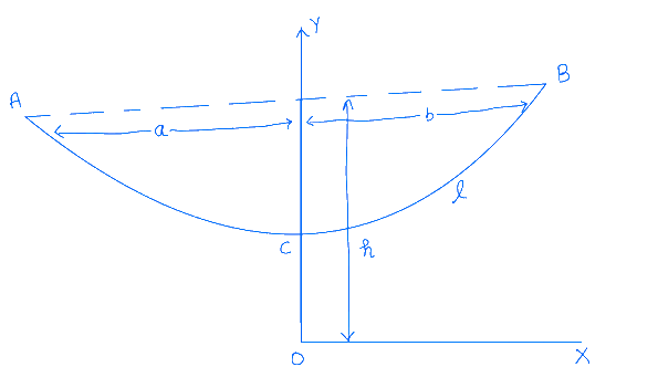
Question:-06(a) A cable of weight w per unit length and length

2 l

hangs from two points

P

and

Q

in the same horizontal line. Show that the span of the cable is

2 l (1 - \frac{2 h^{2}}{3 l^{2}})

, where

h

is the sag in the middle of the tightly stretched position.

Answer:

Introduction

The problem involves a cable of weight

w

per unit length and length

2 l

hanging from two points

P

and

Q

in the same horizontal line. We are asked to show that the span of the cable is

2 l (1 - \frac{2 h^{2}}{3 l^{2}})

, where

h

is the sag in the middle of the tightly stretched position.

Assumptions

The cable hangs from two points $P$ and $Q$ in the same horizontal line.
The length of the cable is $2 l$ .
The sag in the middle of the tightly stretched position is $h$ .

Definitions

$w$ : Weight per unit length of the cable.
$l$ : Half the length of the cable.
$h$ : Sag in the middle of the tightly stretched position.
$c$ : Constant related to the shape of the cable.
$s$ : Arc length along the cable.
$a$ : Span of the cable.

Method/Approach

We will use the equations that describe the shape of the cable and its properties to find the span

a

in terms of

l

and

h

We know that

y^{2} = c^{2} + s^{2}

At the point B,

y = c + h

and

s = l

Therefore

(c + h)^{2} = c^{2} + l^{2}

h^{2} + 2 c h = l^{2}

C = \frac{l^{2} - h^{2}}{2 h} or \frac{l}{c} = \frac{2 l h}{l^{2} - h^{2}} \to (1)

We know that

s = c \sinh (\frac{x}{c})

At the point

B

l = c \sinh (\frac{a}{c})

\frac{l}{c} = \frac{e^{\frac{a}{c}} - e^{- (\frac{a}{2})}}{2} [

by defination,

\sinh x = \frac{1}{2} (e^{x} - e^{- x})]

\frac{2 l}{c} = e^{\frac{a}{c}} - \frac{1}{e^{\frac{a}{2}}}

e^{\frac{2 a}{c}} - 2 \frac{l}{c} e^{\frac{a}{τ}} - 1 = 0

This is a quadratic equation for

e^{\frac{a}{2}}

, whose positive root is given by

e^{\frac{a}{c}} = \frac{l}{c} + \sqrt{\frac{l^{2}}{c^{2}} + 1} or \frac{a}{c} = \log (\frac{l}{c} + \sqrt{1 + \frac{l^{2}}{c^{2}}}) \to (2)

Using (1), we get

1 + \frac{l^{2}}{c^{2}} = 1 + \frac{4 l^{2} h^{2}}{l^{4} + h^{4} - 2 l^{2} h^{2}} = \frac{{(l^{2} + h^{2})}^{2}}{{(l^{2} - h^{2})}^{2}} \to (3)

Therefore,

\frac{l}{c} + \sqrt{1 + \frac{l^{2}}{c^{2}}} = \frac{2 l h}{l^{2} - h^{2}} + \frac{l^{2} + h^{2}}{l^{2} - h^{2}}, b y (1)

and (3)

= \frac{(l + h)^{2}}{l^{2} - h^{2}} = \frac{l + h}{l - h} \to (4)

From (1) , (2) and (4), we obtain

a = \frac{l^{2} - h^{2}}{2 h} \log \frac{l + h}{l - h} \to (5)

We know that, for

| x | < 1

\begin{aligned} \log (1 + x) = x - \frac{x^{2}}{2} + \frac{x^{3}}{3} - \dots, \log (1 - x) = - x - \frac{x^{2}}{2} - \frac{x^{3}}{3} - \dots \\ \log \frac{1 + x}{1 - x} = \log (1 + x) - \log (1 - x) = 2 (x + \frac{x^{3}}{3} + \dots) \to (6) \end{aligned}

Now

\log \frac{l + h}{l - h} = \log \frac{1 + \frac{h}{l}}{1 - \frac{h}{l}} \to

(7)
If the ratio

\frac{h}{l}

is small, then by (6) and (7)

\log \frac{l + h}{l - h} = 2 (\frac{h}{l} + \frac{1}{3} \frac{h^{3}}{l^{3}})

Putting in (5), we obtain

\begin{aligned} a & = \frac{l^{2} - h^{2}}{2 h} \times 2 (\frac{h}{l} + \frac{h^{3}}{3 l^{3}}) = \frac{l^{2} - h^{2}}{l} + \frac{(l^{2} - h^{2}) h^{2}}{3 l^{3}} \\ = l - \frac{h^{2}}{l} + \frac{h^{2}}{3 l} - \frac{1}{3} {(\frac{h}{l})}^{4} \\ = l - \frac{2 h^{2}}{3 l}, neglecting the term {(\frac{h}{l})}^{4} \end{aligned}

Hence

a = l (1 - \frac{2 h^{2}}{3 l^{2}})

Conclusion

We have shown that the span of the cable is

2 l (1 - \frac{2 h^{2}}{3 l^{2}})

, where

h

is the sag in the middle of the tightly stretched position.

Question:-06(b) प्राचल-विचरण विधि का उपयोग करके, निम्नलिखित अवकल समीकरण :

(x^{2} - 1) \frac{d^{2} y}{d x^{2}} - 2 x \frac{d y}{d x} + 2 y = {(x^{2} - 1)}^{2}

को हल कीजिए, जहाँ समानीत समीकरण का एक हल

y = x

दिया गया है ।

Question:-06(b) Solve the following differential equation by using the method of variation of parameters :

(x^{2} - 1) \frac{d^{2} y}{d x^{2}} - 2 x \frac{d y}{d x} + 2 y = {(x^{2} - 1)}^{2}

, given that

y = x

is one solution of the reduced equation.

Answer:

Introduction

We are given a second-order differential equation and one of its solutions. Our task is to find the general solution using the method of variation of parameters.

Assumptions

$y = x$ is a solution of the reduced equation.
We will use the method of variation of parameters to find the general solution.

Definitions

$y$ : Dependent variable
$x$ : Independent variable
$P, Q, R$ : Coefficients in the differential equation
$u, v$ : Variables used in the method of variation of parameters
$w$ : Wronskian determinant
$A, B$ : Constants used in the method of variation of parameters

Method/Approach

We’ll first rewrite the given differential equation in a standard form. Then, we’ll apply the method of variation of parameters to find the general solution.

Work/Calculations

Step 1: Standard Form of Differential Equation

The given equation can be rewritten as:

\frac{d^{2} y}{d x^{2}} - \frac{2 x}{x^{2} - 1} \frac{d y}{d x} + \frac{2}{x^{2} - 1} y = (x^{2} - 1) - - - - (1)

Here,

P = - \frac{2 x}{x^{2} - 1}

Q = \frac{2}{x^{2} - 1}

, and

R = x^{2} - 1

Step 2: Applying Variation of Parameters

We are given that

y = x

is a solution of the reduced equation. Let’s assume

y = u v = x v

Then

v

satisfies:

\frac{d^{2} v}{d x^{2}} + (P + \frac{2}{u} \frac{d u}{d x}) \frac{d v}{d x} = 0

Substituting

P

and

u = x

, we get:

\begin{aligned} \frac{d^{2} v}{d x^{2}} + (- \frac{2 x}{x^{2} - 1} + \frac{2}{x}) \frac{d v}{d x} = 0 \\ \frac{d^{2} v}{d x^{2}} + (- \frac{2}{x (x^{2} - 1)}) \frac{d v}{d x} = 0 Let \frac{d v}{d x} = t \\ \frac{d t}{d x} + [- \frac{2}{x (x^{2} - 1)}] t = 0 \\ \frac{d t}{t} = \frac{2 d x}{x (x^{2} - 1)} \\ \frac{d t}{t} = 2 [- \frac{1}{x} + \frac{1}{2 (x - 1)} + \frac{1}{2 (x + 1)}] \\ \log t = - 2 \log x + \log (x - 1) + \log (x + 1) + \log c_{1} \end{aligned}

\begin{aligned} t = c_{1} (\frac{x^{2} - 1}{x^{2}}) \\ \int d v = \int c_{1} (1 - \frac{1}{x^{2}}) d x \\ v = c_{1} (x + \frac{1}{x}) + c_{2} \\ y_{c} = x [c_{1} (x + \frac{1}{x}) + c_{2}] \\ y_{c} = c_{1} (x^{2} + 1) + c_{2} x \end{aligned}

Let

y_{p} = A u + B v; u = x^{2} + 1, v = x

Then

w = | \begin{array}{cc} x^{2} + 1 & 2 x \\ x & 1 \end{array} | = - x^{2} + 1

Therefore,

A = \int - \frac{V R}{- x^{2} + 1} B = \int \frac{u R}{- x^{2} + 1}

\begin{aligned} A = \int - \frac{(x^{2} - 1) x}{- 1 + x^{2}} d x B = - \int (x^{2} + 1) d x \\ A = \frac{x^{2}}{2} B = - (\frac{x^{3}}{3} + x) \\ y_{p} = \frac{x^{2}}{2} (x^{2} + 1) - (\frac{x^{3}}{3} + x) x \\ y_{p} = \frac{x^{2}}{2} (x^{2} + 1) - x (\frac{x^{3}}{3} + x) \end{aligned}

General solution of (1) is

y = c_{1} (x^{2} + 1) + c_{2} x + \frac{x^{4}}{6} - \frac{x^{2}}{3}

Conclusion

We have successfully solved the given differential equation using the method of variation of parameters. The general solution is

y = c_{1} (x^{2} + 1) + c_{2} x + \frac{x^{4}}{6} - \frac{x^{2}}{3}

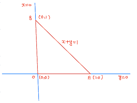
Question:-06(c) समतल में ग्रीन के प्रमेय को

∮_{C} (3 x^{2} - 8 y^{2}) dx + (4 y - 6 xy) dy

के लिए सत्यापित कीजिए, जहाँ

C, x = 0, y = 0, x + y = 1

द्वारा परिभाषित क्षेत्र का सीमा वक्र है ।

Question:-06(c)Verify Green’s theorem in the plane for

∮_{C} (3 x^{2} - 8 y^{2}) d x + (4 y - 6 x y) d y

, where

C

is the boundary curve of the region defined by

x = 0, y = 0

x + y = 1

Answer:

Introduction

We are tasked with verifying Green’s theorem for a given vector field and a specific region in the plane. Green’s theorem relates a line integral around a closed curve

C

to a double integral over the plane region

R

bounded by

C

Assumptions

The curve $C$ is positively oriented.
$C$ is the boundary of the region $R$ , defined by $x = 0$ , $y = 0$ , and $x + y = 1$ .

Definitions

$M = 3 x^{2} - 8 y^{2}$
$N = 4 y - 6 x y$
$R$ : The region bounded by $C$
$C$ : The closed curve consisting of three line segments $O A$ , $A B$ , and $B O$

Theorem

Green’s theorem states that

\iint_{R} (\frac{\partial N}{\partial x} - \frac{\partial M}{\partial y}) d x d y = ∮_{C} (M d x + N d y)

Method/Approach

Calculate $\frac{\partial N}{\partial x} - \frac{\partial M}{\partial y}$ and integrate it over the region $R$ .
Evaluate the line integral $∮_{C} (M d x + N d y)$ along the curve $C$ .
Compare the two results to verify Green’s theorem.

Work/Calculations

Here

M = 3 x^{2} - 8 y^{2}, N = 4 y - 6 x y

The closed curve

C

consists of the straight-line

OA

, the straight-line

AB

and straight-line

BO

. The positive direction is traversing

C

is as shown in the figure and

R

is the region bounded by

c

We have

\iint_{R} (\frac{\partial N}{\partial x} - \frac{\partial M}{\partial y}) d x d y = \iint_{R} [\frac{\partial}{\partial x} (4 y - 2 x y) - \frac{\partial}{\partial y} (3 x^{2} - 8 y^{2})] d x d y

= \iint_{R} [- 6 y + 16 y] d x d y = 10 \iint_{R} y d x d y = 10 \int_{x = 0}^{1} \int_{y = 0}^{1 - x} y d x d y

For the region

R, x

varies from o to 1 and

y

varies from

o

1 - x

= 10 \int_{0}^{1} {[\frac{y^{2}}{2}]}_{y = 0}^{1 - x} d x

, integrating with respect to

y

regarding

x

as constant

= 5 \int_{0}^{1} (1 - x)^{2} d x = 5 \int_{0}^{1} (x - 1)^{2} d x = \frac{5}{3} {[(x - 1)^{3}]}_{0}^{1}

= \frac{5}{3} [0 - (- 1)^{3}] = \frac{5}{3} - - - - (1)

Now let us evaluate the line integral along the curve C. Along the straight-line OA, we have

y = 0, d y = 0

and

x

varies from 0 to 1.

Line integral along

O A = \int_{0}^{1} 3 x^{2} d x = {[x^{3}]}_{0}^{1} = 1

Along the straight-line

AB

, we have

x = 1 - y, d x = - d y

and

y

varies from 0 to 1

Line integral along

AB

\begin{aligned} = \int_{0}^{1} [{3 (1 - y)^{2} 8 y^{2}} (- d y) + {4 y - 6 y (1 - y)} d y] \\ = \int_{0}^{1} [- 3 (1 - 2 y + y^{2}) + 8 y^{2} + 4 y - 6 y + 6 y^{2}] d y \\ = \int_{0}^{1} (11 y^{2} + 4 y - 3) d y = {[\frac{11}{3} y^{3} + 2 y^{2} - 3 y]}_{0}^{1} = \frac{8}{3} \end{aligned}

Along the straight-line

BO

, we have

x = 0, d x = 0

and

y

varies from 1 to 0

Line integral along

B O = \int_{1}^{3} 4 y d y = 2 {[y^{2}]}_{1}^{0} = - 2

Total line integral along the closed curve

C

= 1 + \frac{8}{3} - 2 = \frac{5}{3} \to (2)

From (1) and (2), we see that Green’s theorem is verified

Step 3: Verification

Both the double integral over

R

and the line integral along

C

yield

\frac{5}{3}

, verifying Green’s theorem.

Conclusion

We have successfully verified Green’s theorem for the given vector field and region. Both the double integral over the region

R

and the line integral along the curve

C

resulted in

\frac{5}{3}

, confirming that Green’s theorem holds in this case.

Question:-07(a) स्टोक्स प्रमेय को

\vec{F} = x \hat{i} + z^{2} \hat{j} + y^{2} \hat{k}

के लिए प्रथम अष्टांशक में स्थित समतल पृष्ठ :

x + y + z = 1

पर सत्यापित कीजिए ।

Question:-07(a) Verify Stokes’ theorem for

\vec{F} = x \hat{i} + z^{2} \hat{j} + y^{2} \hat{k}

over the plane surface :

x + y + z = 1

lying in the first octant.

Answer:

Introduction:

In this analysis, we aim to verify Stokes’ theorem for the given vector field

\vec{F} = x \hat{i} + z^{2} \hat{j} + y^{2} \hat{k}

over a specific plane surface. Stokes’ theorem relates the circulation of a vector field along a closed curve to the flux of its curl through a surface bounded by that curve. The surface of interest is defined by

x + y + z = 1

and lies in the first octant.

The problem at hand is to verify Stokes’ theorem for the given vector field

\vec{F} = x \hat{i} + z^{2} \hat{j} + y^{2} \hat{k}

over the plane surface defined by

x + y + z = 1

in the first octant.

Stokes’ theorem states that:

∮_{C} \vec{F} \cdot d \vec{r} = \iint_{S} (\nabla \times \vec{F}) \cdot \hat{n} d s (Equation 1)

Calculate the Curl of $\vec{F}$

The curl of

\vec{F}

is given by:

\nabla \times \vec{F} = | \begin{array}{ccc} \hat{i} & \hat{j} & \hat{k} \\ \frac{\partial}{\partial x} & \frac{\partial}{\partial y} & \frac{\partial}{\partial z} \\ x & z^{2} & y^{2} \end{array} |

This simplifies to

2 (y - z) \hat{i}

Calculate the Unit Normal Vector $\hat{n}$

The surface is defined by

ϕ = x + y + z - 1 = 0

. The gradient of

ϕ

\nabla ϕ = \hat{i} + \hat{j} + \hat{k}

The unit normal vector

\hat{n}

is:

\hat{n} = \frac{\nabla ϕ}{| \nabla ϕ |} = \frac{\hat{i} + \hat{j} + \hat{k}}{\sqrt{3}}

Calculate $d s$

The differential area element

d s

is given by:

d s = \frac{d x d y}{| \hat{n} \cdot \hat{k} |} = \frac{d x d y}{\frac{1}{\sqrt{3}}}

Calculate $\iint_{S} (\nabla \times \vec{F}) \cdot \hat{n} d s$

(\nabla \times \vec{F}) \cdot \hat{n} d s = 2 (y - z) d x d y

Substitute

z = 1 - x - y

= 2 [y - (1 - x - y)] d x d y

= 2 [2 y + x - 1] d x d y

Now, integrate this over the region

R

defined by

x : 0 \to 1

and

y : 0 \to 1 - x

2 \int_{x = 0}^{1} [\int_{y = 0}^{1 - x} (2 y + x - 1) d y] d x

First, integrate with respect to

y

\int (2 y + x - 1) d y = 2 \frac{y^{2}}{2} + x y - y = y^{2} + x y - y

Now, evaluate this integral from

y = 0

y = 1 - x

{[y^{2} + x y - y]}_{y = 0}^{1 - x} = (1 - x)^{2} + x (1 - x) - (1 - x) = (1 - x)^{2} + x - x^{2} - 1 + x = (1 - x)^{2} - x^{2}

Now, integrate this result with respect to

x

2 \int_{x = 0}^{1} ((1 - x)^{2} - x^{2}) d x

= 2 \int_{x = 0}^{1} (1 - 2 x + x^{2} - x^{2}) d x

= 2 \int_{x = 0}^{1} (1 - 2 x) d x

= 2 {[x - x^{2}]}_{x = 0}^{1} = 2 (1 - 1) = 0

Line Integral Along $A B$

Along

A B

x + y = 1

and

z = 0

. Let

x = t

, then

y = 1 - t

\int_{A B} \vec{F} \cdot d \vec{r} = \int_{t = 1}^{0} t d t = - \frac{1}{2}

Line Integral Along $B C$

Along

B C

y + z = 1

and

x = 0

. Let

y = t

, then

z = 1 - t

\int_{B C} \vec{F} \cdot d \vec{r} = \int_{t = 1}^{0} (1 - 2 t) d t = 0

Line Integral Along $C A$

Along

C A

x + z = 1

and

y = 0

. Let

x = t

, then

z = 1 - t

\int_{C A} \vec{F} \cdot d \vec{r} = \int_{t = 0}^{1} t d t = \frac{1}{2}

Sum of Line Integrals

∮_{C} \vec{F} \cdot d \vec{r} = \int_{A B} \vec{F} \cdot d \vec{r} + \int_{B C} \vec{F} \cdot d \vec{r} + \int_{C A} \vec{F} \cdot d \vec{r} = - \frac{1}{2} + 0 + \frac{1}{2} = 0

Conclusion:

After carefully evaluating both sides of Stokes’ theorem, we find that the line integral of

\vec{F}

around the closed curve

C

is equal to zero. This is in agreement with the flux of

\nabla \times \vec{F}

through the surface

S

. Therefore, we have successfully verified Stokes’ theorem for the given vector field and surface in the first octant.

Question:-07(b) लाप्लास रूपांतरण का उपयोग करके निम्नलिखित प्रारंभिक मान समस्या :

\frac{d^{2} y}{{dt}^{2}} - 3 \frac{dy}{dt} + 2 y = h (t)

, जहाँ

h (t) = {\begin{array}{cc} 2, & 0 < t < 4, \\ 0, & t > 4, \end{array} y (0) = 0, y^{'} (0) = 0

को हल कीजिए।

Question:-07(b) Solve the following initial value problem by using Laplace’s transformation

\frac{d^{2} y}{{dt}^{2}} - 3 \frac{dy}{dt} + 2 y = h (t)

, where

h (t) = {\begin{array}{cc} 2, & 0 < t < 4, \\ 0, & t > 4, \end{array} y (0) = 0, y^{'} (0) = 0

Answer:

Introduction

The problem is an initial value problem (IVP) involving a second-order linear ordinary differential equation (ODE) with a piecewise-defined forcing function

h (t)

. The equation is:

\frac{d^{2} y}{d t^{2}} - 3 \frac{d y}{d t} + 2 y = h (t)

The initial conditions are

y (0) = 0

and

y^{'} (0) = 0

. The function

h (t)

is defined as:

h (t) = {\begin{cases} 2, & 0 < t < 4, \\ 0, & t > 4 \end{cases}

We will use Laplace’s transformation to solve this problem. Let’s go through it step-by-step to understand it thoroughly.

Work/Calculations

Step 1: Take the Laplace Transform of Both Sides

The Laplace transform of the given ODE is:

L {\frac{d^{2} y}{d t^{2}}} - 3 L {\frac{d y}{d t}} + 2 L {y} = L {h (t)}

Using the properties of Laplace transforms, we get:

s^{2} Y (s) - s y (0) - y^{'} (0) - 3 (s Y (s) - y (0)) + 2 Y (s) = H (s)

Let’s substitute the initial conditions

y (0) = 0

and

y^{'} (0) = 0

s^{2} Y (s) - 0 - 0 - 3 (s Y (s) - 0) + 2 Y (s) = H (s)

After simplifying, we get:

(s^{2} - 3 s + 2) Y (s) = H (s)

Step 2: Find $H (s)$

The function

h (t)

is piecewise-defined. It can be represented as

h (t) = 2 u (t) - 2 u (t - 4)

, where

u (t)

is the unit step function.

The Laplace transform of

h (t)

is:

H (s) = 2 L {u (t)} - 2 L {u (t - 4) e^{- 4 s}}

After calculating, we get:

H (s) = \frac{2}{s} - \frac{2 e^{- 4 s}}{s}

Step 3: Solve for $Y (s)$

Substitute

H (s)

into the equation:

(s^{2} - 3 s + 2) Y (s) = \frac{2}{s} - \frac{2 e^{- 4 s}}{s}

Combine like terms:

Y (s) (s^{2} - 3 s + 2) = \frac{2}{s} - \frac{2 e^{- 4 s}}{s}

Solve for

Y (s)

Y (s) = \frac{\frac{2}{s} - \frac{2 e^{- 4 s}}{s}}{s^{2} - 3 s + 2}

After simplifying, we get:

Y (s) = \frac{2 (1 - e^{- 4 s})}{s (s - 1) (s - 2)}

This can be further simplified to:

Y (s) = (1 - e^{- 4 s}) [\frac{1}{s} - \frac{2}{s - 1} + \frac{1}{s - 2}]

Step 4: Detailed Inverse Laplace Transform

This can be broken down into two parts for easier inverse Laplace transformation:

Y (s) = [\frac{1}{s} - \frac{2}{s - 1} + \frac{1}{s - 2}] - [\frac{e^{- 4 s}}{s} + \frac{2 e^{- 4 s}}{s - 1} + \frac{e^{- 4 s}}{s - 2}]

Inverse Laplace Transform of the First Part

The inverse Laplace transform of

\frac{1}{s} - \frac{2}{s - 1} + \frac{1}{s - 2}

is straightforward:

L^{- 1} {\frac{1}{s} - \frac{2}{s - 1} + \frac{1}{s - 2}} = 1 - 2 e^{t} + e^{2 t}

Inverse Laplace Transform of the Second Part

The inverse Laplace transform of

\frac{e^{- 4 s}}{s} + \frac{2 e^{- 4 s}}{s - 1} + \frac{e^{- 4 s}}{s - 2}

involves exponential-shift theorems:

L^{- 1} {\frac{e^{- 4 s}}{s} + \frac{2 e^{- 4 s}}{s - 1} + \frac{e^{- 4 s}}{s - 2}} = u (t - 4) + 2 e^{(t - 4)} - e^{2 (t - 4)}

Here,

u (t - 4)

is a unit step function that becomes 1 for

t \geq 4

and is zero for

t < 4

. It "turns on" the terms

2 e^{t - 4} - e^{2 t - 4}

when

t \geq 4

, reflecting the change in

h (t)

at that time.

Combine Both Parts

Combining both parts, we get:

y (t) = (1 - 2 e^{t} + e^{2 t}) - (u (t - 4) + 2 e^{(t - 4)} - e^{2 (t - 4)})

After simplifying, we get:

y (t) = {\begin{matrix} e^{2 t} - 2 e^{t} + 2 e^{t - 4} - e^{2 t - 4}; t > 4 \\ e^{2 t} - 2 e^{t} + 1; t < 4 \end{matrix}

Conclusion

The solution to the initial value problem is:

y (t) = {\begin{matrix} e^{2 t} - 2 e^{t} + 2 e^{t - 4} - e^{2 t - 4}; t > 4 \\ e^{2 t} - 2 e^{t} + 1; t < 4 \end{matrix}

This function satisfies the given differential equation and initial conditions. We’ve gone through each step in detail, including the inverse Laplace transform and the role of the unit step function

u (t - 4)

, to arrive at the final solution.

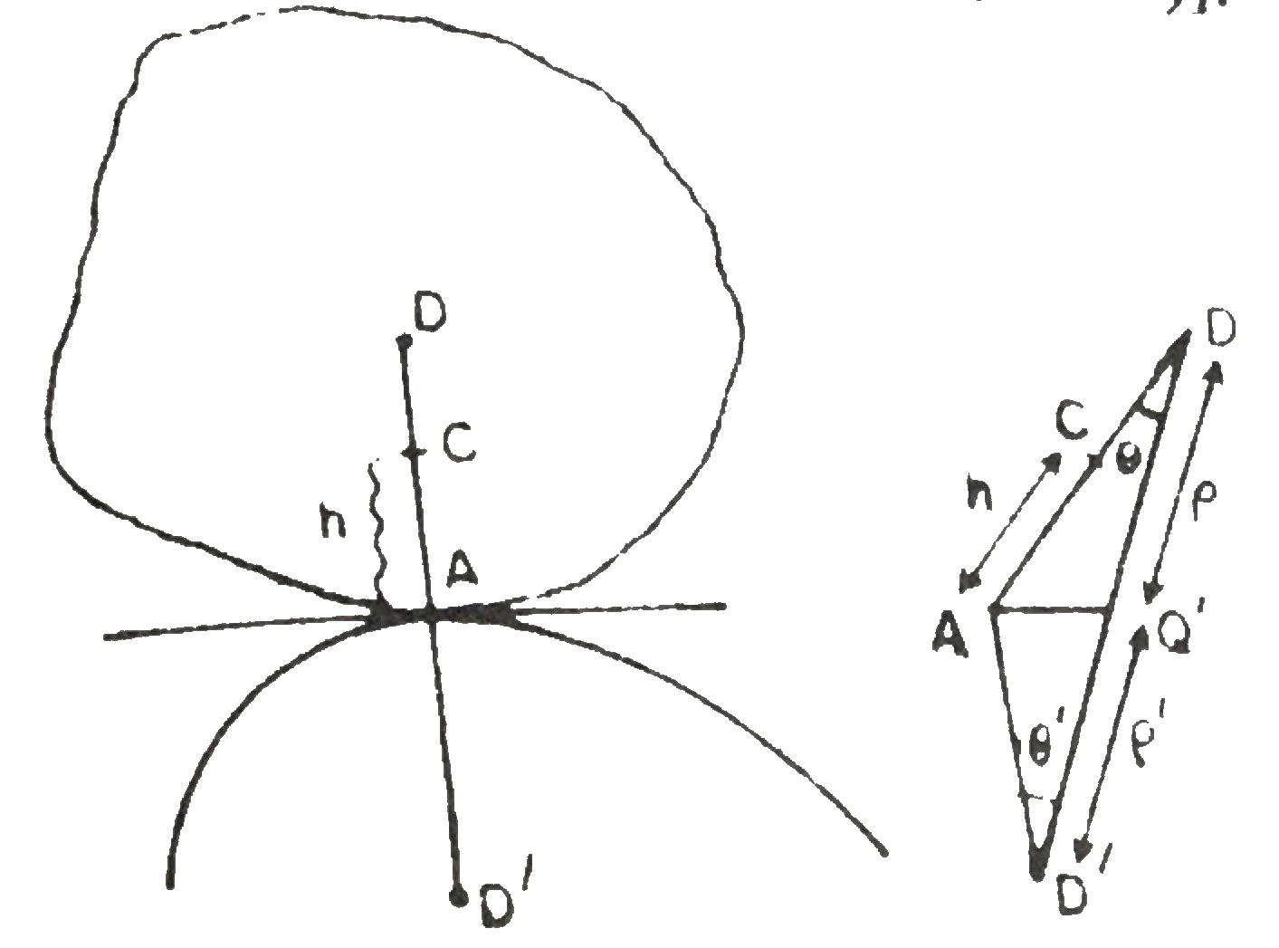
Question:-07(c) माना किसी भी अनुप्रस्थ-काट का एक बेलन दूसरे स्थिर बेलन पर संतुलित है, जहाँ वक्रीय पृष्ठों का संस्पर्श रूक्ष है तथा उभयनिष्ठ स्पर्श-रेखा क्षैतिज है । माना दोनों बेलनों के स्पर्श बिन्दु पर उनकी वक्रता त्रिज्याएँ

ρ

तथा

ρ^{'}

हैं और संस्पर्श बिन्दु से ऊपरी बेलन के गुरुत्व केन्द्र की ऊँचाई

h

है । दर्शाइए कि स्थायी साम्य में ऊपरी बेलन संतुलित है यदि

h < \frac{ρ ρ^{'}}{ρ + ρ^{'}}

।

Question:-07(c) Suppose a cylinder of any cross-section is balanced on another fixed cylinder, the contact of curved surfaces being rough and the common tangent line horizontal. Let

ρ

and

ρ^{'}

be the radii of curvature of the two cylinders at the point of contact and

h

be the height of centre of gravity of the upper cylinder above the point of contact. Show that the upper cylinder is balanced in stable equilibrium if

h < \frac{ρ ρ^{'}}{ρ + ρ^{'}}

Answer:

Introduction

The problem is about two cylinders in contact with each other. One cylinder is balanced on top of another fixed cylinder. The point where they touch is called the point of contact. The problem asks us to show that the upper cylinder is in stable equilibrium under certain conditions. Specifically, we need to prove that the upper cylinder will be stable if the height

h

of its center of gravity above the point of contact is less than

\frac{ρ ρ^{'}}{ρ + ρ^{'}}

, where

ρ

and

ρ^{'}

are the radii of curvature for the two cylinders at the point of contact.

Work/Calculations

Step 1: Define Variables and Initial Conditions

Let

D

and

D^{'}

be the centers of curvature of the sections of the cylinders at the point of contact

A

. Then

A D = ρ

and

A D^{'} = ρ^{'}

. Let

A C = h

, where

C

is the center of gravity of the upper cylinder.

Step 2: Displacement of the Upper Cylinder

Suppose the upper cylinder is slightly displaced, and the point of contact

A

moves through a small angle

θ^{'}

about

D^{'}

. The line

D C

makes a small angle

θ

with

D D^{'}

Since

θ

and

θ^{'}

are small, we can approximate the sections near

A

as circular arcs with radii

ρ

and

ρ^{'}

. Therefore, we have:

ρ θ = ρ^{'} θ^{'} (Equation 1)

Step 3: Calculate the Height of the Center of Gravity $G$

The height of the center of gravity

G

above

D^{'}

is given by:

[(ρ + ρ^{'}) \cos θ^{'} - (ρ - h) \cos (θ + θ^{'})]

Step 4: Calculate the Potential Energy $V$

The potential energy

V

of the upper cylinder is:

V = W [(ρ + ρ^{'}) \cos θ^{'} - (ρ - h) \cos (θ + θ^{'})]

Let’s substitute the values:

V = W [(ρ + ρ^{'}) (1 - \frac{1}{2} θ^{' 2}) - (ρ - h) (1 - \frac{1}{2} {(θ + θ^{'})}^{2})]

After calculating, we get:

V = W [\frac{1}{2} (ρ - h) {(θ + θ^{'})}^{2} - \frac{1}{2} (ρ + ρ^{'}) θ^{' 2}] + C

where

C

is a constant.

Step 5: Further Simplification Using Equation 1

V = \frac{1}{2} W [(ρ - h) {(\frac{ρ^{'} θ^{'}}{ρ} + θ^{'})}^{2} - (ρ + ρ^{'}) θ^{' 2}] + C

After obtaining the expression for

V

, there are additional steps to simplify it further. Using Equation 1, we can rewrite

V

as:

V = \frac{1}{2} W θ^{' 2} [(ρ - h) {(1 + \frac{ρ^{'}}{ρ})}^{2} - (ρ^{'} + ρ)] + C

After calculating, we get:

V = \frac{1}{2} W θ^{' 2} {[\frac{ρ + ρ^{'}}{ρ}]}^{2} [(ρ - h) - \frac{ρ^{2}}{ρ + ρ^{'}}] + C

Finally, we arrive at:

V = \frac{1}{2} W θ^{' 2} {[\frac{ρ + ρ^{'}}{ρ}]}^{2} [\frac{ρ ρ^{'}}{ρ + ρ^{'}} - h] + C

Step 6: Conditions for Stable Equilibrium

For stable equilibrium,

\frac{d V}{d θ^{'}} = 0

and

\frac{d^{2} V}{d θ^{' 2}} > 0

\frac{d V}{d θ^{'}} = W {(\frac{ρ + ρ^{'}}{ρ})}^{2} θ^{'} [\frac{ρ ρ^{'}}{ρ + ρ^{'}} - h]

\frac{d^{2} V}{d θ^{' 2}} = W {(\frac{ρ + ρ^{'}}{ρ})}^{2} [\frac{ρ ρ^{'}}{ρ + ρ^{'}} - h]

Now, for

θ^{'} = 0

, the first derivative

\frac{d V}{d θ^{'}} = 0

, indicating that it is a position of equilibrium.

Also, at

θ^{'} = 0

, the second derivative

\frac{d^{2} V}{d θ^{' 2}} > 0

\frac{ρ ρ^{'}}{ρ + ρ^{'}} > h

This confirms that

h < \frac{ρ ρ^{'}}{ρ + ρ^{'}}

for stable equilibrium.

Conclusion

We have shown that the upper cylinder will be in stable equilibrium if the height

h

of its center of gravity above the point of contact is less than

\frac{ρ ρ^{'}}{ρ + ρ^{'}}

. This was achieved by calculating the potential energy, simplifying it, and applying conditions for stable equilibrium.

Question:-08(a) (i) अवकल समीकरण :

(x^{2} - a^{2}) p^{2} - 2 xyp + y^{2} + a^{2} = 0

, जहाँ

p = \frac{dy}{dx}

, के व्यापक व विचित्र हलों को ज्ञात कीजिए । व्यापक व विचित्र हलों के बीच ज्यामितीय संबंध को भी दीजिए ।

Question8(a) (i) Find the general and singular solutions of the differential equation:

(x^{2} - a^{2}) p^{2} - 2 x y p + y^{2} + a^{2} = 0

, where

p = \frac{d y}{d x}

. Also give the geometric relation between the general and singular solutions.

Answer:

Introduction

The problem asks us to find both the general and singular solutions of a given differential equation

(x^{2} - a^{2}) p^{2} - 2 x y p + y^{2} + a^{2} = 0

, where

p = \frac{d y}{d x}

. Additionally, we are asked to describe the geometric relationship between these solutions.

Work/Calculations

Step 1: Given Differential Equation

The differential equation provided is:

(x^{2} - a^{2}) p^{2} - 2 x y p + y^{2} + a^{2} = 0 (Equation 1)

Step 2: Simplify the Equation

Let’s simplify Equation 1:

x^{2} p^{2} - 2 x y p + y^{2} - a^{2} p^{2} + a^{2} = 0

Combine like terms:

(x p - y)^{2} + a^{2} (1 - p^{2}) = 0

Further simplification gives:

(x p - y)^{2} = a^{2} (p^{2} - 1)

Finally, we get:

x p - y = \pm a \sqrt{p^{2} - 1}

So, we have:

y = x p \pm a \sqrt{p^{2} - 1}

Step 3: General Solution in Clairaut’s Form

The equation is in Clairaut’s form, and its general solution is:

y = x c \pm a \sqrt{c^{2} - 1} (Equation 2)

Step 4: Finding the p-discriminant

To find the p-discriminant, we use

B^{2} - 4 A C = 0

(since the given ODE is a quadratic equation):

(4 x y)^{2} - 4 (x^{2} - a^{2}) (y^{2} + a^{2}) = 0

Simplifying, we get:

x^{2} y^{2} - (x^{2} - a^{2}) (y^{2} + a^{2}) = 0

Further simplification leads to:

x^{2} - y^{2} = a^{2} (Equation 3)

Step 5: Singular Solution and Geometric Relation

Equation 3 is the same as the c-discriminant and satisfies the given ODE. Therefore, Equation 3 is the singular solution of Equation 1. The geometric relation between the general and singular solutions is that they are envelopes of each other, represented by a hyperbola curve.

Conclusion

We found both the general and singular solutions for the given differential equation. The general solution is

y = x c \pm a \sqrt{c^{2} - 1}

, and the singular solution is

x^{2} - y^{2} = a^{2}

. The geometric relationship between these solutions is that they are envelopes of each other, represented by a hyperbola curve.

Question:-08(a) (ii) निम्नलिखित अवकल समीकरण को हल कीजिए :

(3 x + 2)^{2} \frac{d^{2} y}{d x^{2}} + 5 (3 x + 2) \frac{d y}{d x} - 3 y = x^{2} + x + 1

Question:-08(a) (ii) Solve the following differential equation :

(3 x + 2)^{2} \frac{d^{2} y}{d x^{2}} + 5 (3 x + 2) \frac{d y}{d x} - 3 y = x^{2} + x + 1

Answer:

Given equation:

\begin{aligned} (3 x + 2)^{2} \frac{d^{2} y}{d x^{2}} + 5 (3 x + 2) \frac{d y}{d x} - 3 y = x^{2} + x + 1 \to (1) \\ \Rightarrow \frac{d^{2} y}{d x^{2}} + \frac{5}{3 x + 2} \frac{d y}{d x} - \frac{3}{3 x + 2} y = \frac{x^{2} + x + 1}{(3 x + 2)^{2}} [D \equiv \frac{d}{d t}] \\ Let (3 x + 2) \\ \Rightarrow z = \log (3 x + 2) \\ [9 D (D - 1) + 5 \times 3 D - 3] y = {(\frac{e^{z} - 2}{3})}^{2} + (\frac{e^{z} - 2}{3}) + 1 \\ \Rightarrow [9 (D^{2} - D) + 15 D - 3] y = e^{2 z} - 4 e^{z} + 4 + 3 (e^{z} - 2) + 9 \\ \Rightarrow (9 D^{2} + 6 D - 3) y = e^{2 z} - e^{z} + 7 \to (2) \end{aligned}

Auxiliary equation:

\begin{aligned} 9 m^{2} + 6 m - 3 = 0 \\ \Rightarrow 9 m^{2} + 9 m - m - 3 = 0 \\ \Rightarrow m = - 1, \frac{1}{3} \end{aligned}

Therefore, the Complementary Function (C.F.) is:

y_{C . F} = C_{1} e^{- z} + C_{2} e^{\frac{z}{3}} \to (3)

Particular Integral (P.I.):

\begin{aligned} And y_{P . I} = \frac{e^{2 z} - e^{z} + 7}{9 D^{2} + 6 D - 3} \\ y_{p} = \frac{e^{2 z}}{9 \times 4 + 6 \times 2 - 3} - \frac{e^{z}}{9 + 6 - 3} + \frac{7}{- 3} \\ \Rightarrow y_{p} = \frac{e^{2 z}}{36 + 12 - 3} - \frac{e^{z}}{12} - \frac{7}{3} \\ \Rightarrow y_{p} = \frac{e^{2 z}}{45} - \frac{e^{z}}{12} - \frac{7}{3} \to (4) \end{aligned}

Overall solution:

\begin{aligned} y = y_{c} + y_{p} \\ \Rightarrow y = c_{1} e^{- z} + c_{2} e^{\frac{z}{3}} + \frac{e^{2 z}}{45} - \frac{e^{z}}{12} - \frac{7}{3} \\ \Rightarrow y = \frac{c_{1}}{3 x + 2} + c_{2} (3 x + 2)^{\frac{1}{3}} + \frac{36 x^{2} + 3 x - 434}{180} \end{aligned}

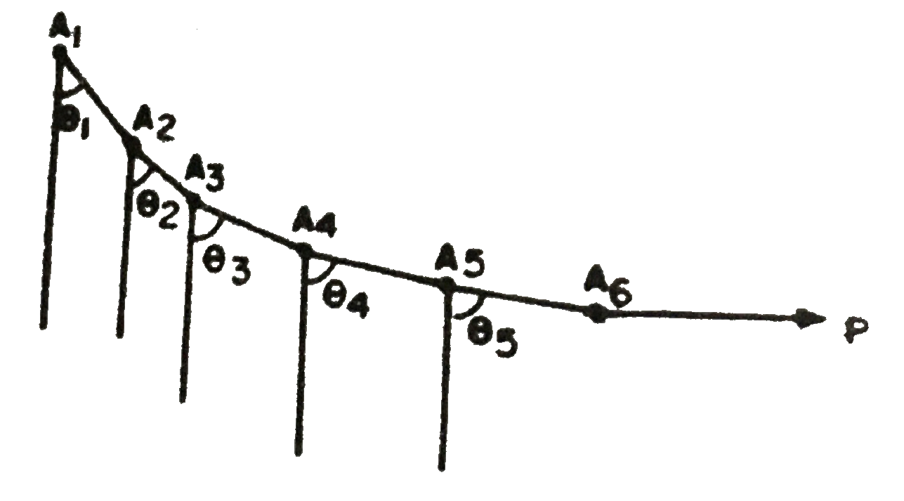
Question:-08(b)

n

बराबर एकसमान छड़ों की एक श्रृंखला एक-दूसरे के साथ चिकने रूप से जुड़ी हुई है तथा इसके एक सिरे

A_{1}

से लटकी हुई है । एक क्षैतिज बल

\vec{P}

शृंखला के दूसरे सिरे

A_{n + 1}

पर लगाया गया है । साम्य विन्यास में अधोमुखी ऊर्ध्वाधर रेखा से छड़ों के झुकाव ज्ञात कीजिए ।

Question:-08(b) A chain of

n

equal uniform rods is smoothly jointed together and suspended from its one end

A_{1}

. A horizontal force

\vec{P}

is applied to the other end

A_{n + 1}

of the chain. Find the inclinations of the rods to the downward vertical line in the equilibrium configuration.

Answer:

Consider a chain of

n

equal uniform rods smoothly jointed together and suspended from one end (denoted as

A_{1}

). A horizontal force

\vec{P}

is applied to the other end (

A_{n + 1}

) of the chain. We need to find the inclinations of the rods to the downward vertical line in the equilibrium configuration.

Each rod has length

2 a

and weight

w

. The potential energy in a general configuration is given by:

V = - w a \cos θ_{1} - w (2 a \cos θ_{1} + a \cos θ_{2}) - \dots

- w (2 a \cos θ_{1} + 2 a \cos θ_{2} + \dots + 2 a \cos θ_{n - 1} + a \cos θ_{n})

= - w a [(2 n - 1) \cos θ_{1} + (2 n - 3) \cos θ_{2} + \dots + 3 \cos θ_{n - 1} + \cos θ_{n}]

In a small virtual displacement, the work done

δ W_{1}

is given by:

\begin{aligned} δ W_{1} & = w a δ [(2 n - 1) \cos θ_{1} + (2 n - 3) \cos θ_{2} + \dots + 3 \cos θ_{n - 1} + \cos δ θ_{n}] \\ = - w a [(2 n - 1) \sin θ_{1} δ θ_{1} + (2 n - 3) \sin θ_{2} δ θ_{2} + \dots \\ + 3 \sin θ_{n - 1} δ θ_{n - 1} + \sin θ_{n} δ θ_{n}] \end{aligned}

The work done by the force

P

is given by

δ W_{2}

\begin{aligned} δ W_{2} & = P \times Horizontal displacement of A_{n + 1} \\ = P δ (2 a \sin θ_{1} + 2 a \sin θ_{2} + \dots + 2 a \sin θ_{n}) \\ = 2 P a (\cos θ_{1} δ θ_{1} + \cos θ_{2} δ θ_{2} + \dots + \cos θ_{n} δ θ_{n}) \end{aligned}

The total work done

δ W

is the sum of

δ W_{1}

and

δ W_{2}

δ W = δ W_{1} + δ W_{2}

Using the expressions for

δ W_{1}

and

δ W_{2}

in the equation above, we get:

δ W = [2 P \cos θ_{1} - (2 n - 1) w \sin θ_{1}] a δ θ_{1} + [2 P \cos θ_{2} - (2 n - 3) w \sin θ_{2}] a δ θ_{2} + \dots + [2 P \cos θ_{n} - w \sin θ_{n}] a δ θ_{n} = 0

For the equilibrium position,

δ W = 0

, which leads to the following equations:

\begin{aligned} 2 P \cos θ_{1} - (2 n - 1) w \sin θ_{1} & = 0 \\ 2 P \cos θ_{2} - (2 n - 3) w \sin θ_{2} & = 0 \\ 2 P \cos θ_{n} - w \sin θ_{n} & = 0 \end{aligned}

Hence, the inclinations of the rods to the downward vertical in the equilibrium configuration are given by:

\tan θ_{1} = \frac{2 P}{w (2 n - 1)}, \tan θ_{2} = \frac{2 P}{w (2 n - 3)}, \dots, \tan θ_{n} = \frac{2 P}{w}

Question:-08(c) गाउस के अपसरण प्रमेय का उपयोग करके

\iint_{S} \vec{F} \cdot \vec{n} dS

का मान निकालिए, जहाँ

\vec{F} = x \hat{i} - y \hat{j} + (z^{2} - 1) \hat{k}

तथा

S

, पृष्ठों

z = 0, z = 1, x^{2} + y^{2} = 4

द्वारा बना हुआ बेलन है ।

Question:-08(c) Using Gauss’ divergence theorem, evaluate

\iint_{S} \vec{F} \cdot \vec{n} d S

, where

\vec{F} = x \hat{i} - y \hat{j} + (z^{2} - 1) \hat{k}

and

S

is the cylinder formed by the surfaces

z = 0, z = 1, x^{2} + y^{2} = 4

Answer:

Step 1 – Gauss’ Divergence Theorem:

We begin by applying Gauss’ Divergence Theorem, which connects the surface integral to a triple integral:

\iint_{S} \vec{F} \cdot \vec{n} d S = ∭_{V} div \vec{F} d V

Step 2 – Divergence Calculation:

We calculate the divergence of

\vec{F}

by taking partial derivatives:

div \vec{F} = \frac{\partial}{\partial x} (x) + \frac{\partial}{\partial y} (- y) + \frac{\partial}{\partial z} (z^{2} - 1) = 1 - 1 + 2 z = 2 z

This gives us the expression for the divergence of

\vec{F}

Step 3 – Triple Integral Setup:

Next, we set up the triple integral to calculate

∭_{V} div \vec{F} d V

. We integrate with respect to

z

from 0 to 1,

y

from -2 to 2, and

x

from

- \sqrt{4 - y^{2}}

\sqrt{4 - y^{2}}

Step 4 – Integral Calculation (Part 1):

We start by integrating with respect to

x

from

- \sqrt{4 - y^{2}}

\sqrt{4 - y^{2}}

\int_{x = - \sqrt{4 - y^{2}}}^{\sqrt{4 - y^{2}}} 2 z d x = 4 z \sqrt{4 - y^{2}}

Step 5 – Integral Calculation (Part 2):

Continuing, we integrate with respect to

y

from -2 to 2, considering the expression

\sqrt{4 - y^{2}}

\begin{aligned} \int_{y = - 2}^{2} 4 z \sqrt{4 - y^{2}} d y \\ = 4 z \int_{y = - 2}^{2} \sqrt{4 - y^{2}} d y \end{aligned}

Step 6 – Integral Calculation (Part 3):

Finally, we integrate with respect to

z

from 0 to 1:

\begin{aligned} \int_{z = 0}^{1} 4 z \int_{y = - 2}^{2} \sqrt{4 - y^{2}} d y d z \\ = \int_{z = 0}^{1} 4 z {[2 \sin^{- 1} (\frac{y}{2})]}_{y = - 2}^{2} d z \\ = 4 \int_{z = 0}^{1} 2 z [\sin^{- 1} (1) - \sin^{- 1} (- 1)] d z \\ = 4 \int_{z = 0}^{1} 2 z [\frac{π}{2} - (- \frac{π}{2})] d z \\ = 4 \int_{z = 0}^{1} 2 z \cdot π d z \\ = 8 π \int_{z = 0}^{1} z d z \\ = 8 π {[\frac{z^{2}}{2}]}_{z = 0}^{1} \\ = 4 π \end{aligned}

Therefore, the evaluated surface integral

\iint_{S} \vec{F} \cdot \vec{n} d S

is indeed

4 π

Free UPSC Mathematics Optional Paper-1 2022 Solutions: View Online | UPSC Maths Solution | IAS Maths Solution

Given:

Proof:

Step 1: S S SSS is Linearly Independent (Given)

Step 2: S S SSS Spans V V VVV

Conclusion

Summary:

Concept:

Calculation:

Introduction

Assumptions

Method/Approach

Work/Calculations

Step 1: Convert to Augmented Matrix

Step 2: Row Reduction to RREF

First Row Operation

Second Row Operation

Third Row Operation

Fourth Row Operation

Fifth Row Operation

Step 3: Back-Substitution

Conclusion

Introduction

Assumptions

Definitions

Constraints

Objective Function

Method/Approach

Work/Calculations

Partial Derivatives

Substitute into Objective Function

Conclusion

Introduction

Definitions

Method/Approach

Work/Calculations

Step 1: Equation of Plane P ′ Q ′ R ′ P ′ Q ′ R ′ P^(‘)Q^(‘)R^(‘)P’Q’R’P′Q′R′

Step 2: Coordinates of the Feet of the Normals

Step 3: Comparison with Ellipsoid Equation

Step 4: Substituting into Equation (1)

Conclusion

Introduction

Definitions

Method/Approach

Work/Calculations

Part (i): Proving P P PPP is a Subspace

Part (ii): Finding a Basis and Dimension

Conclusion

Setting up the Double Integral

Conclusion

Introduction

Assumptions

Definitions

Method/Approach

Work/Calculations

Step 1: Parametric Equations for the Lines

Step 2: Distance Between the Lines

Step 3: Radius of the Smallest Sphere

Step 4: Coordinates of the Center

Conclusion

Introduction

Assumptions

Definition

Method/Approach

Finding the Linear Map T T T\mathrm{T}T

Proving No Real Eigenvalues for θ = π 2 θ = π 2 theta=(pi)/(2)\theta = \frac{\pi}{2}θ=π2

Work/Calculations

Step 1: Substituting θ = π 2 θ = π 2 theta=(pi)/(2)\theta = \frac{\pi}{2}θ=π2 into A A AAA

Step 2: Finding the Characteristic Equation

Conclusion

Introduction

Assumptions

Method/Approach

1. Symmetry

2. Curve Passing Through Origin

3. Intercepts with Coordinate Axes

4. Asymptotes

5. Region

Conclusion

Introduction

Step 1: $S$ is Linearly Independent (Given)

Step 2: $S$ Spans $V$

Step 1: Equation of Plane $P^{'} Q^{'} R^{'}$

Part (i): Proving $P$ is a Subspace

Finding the Linear Map $T$

Proving No Real Eigenvalues for $θ = \frac{π}{2}$

Step 1: Substituting $θ = \frac{π}{2}$ into $A$

Calculate the Curl of $\vec{F}$

Calculate the Unit Normal Vector $\hat{n}$

Calculate $d s$

Calculate $\iint_{S} (\nabla \times \vec{F}) \cdot \hat{n} d s$

Line Integral Along $A B$

Line Integral Along $B C$

Line Integral Along $C A$

Step 2: Find $H (s)$

Step 3: Solve for $Y (s)$