Question:-1(a)
Design and develop an efficient algorithm to find the list of prime numbers in the range 501 to 2000. What is the complexity of this algorithm?
Answer:
🔍 Sieve of Eratosthenes Algorithm for Primes (501 to 2000)
🧠 Step 1: Algorithm Design
- Create a boolean list
is_prime[0..2000], initialize all entries asTrue. - Mark
is_prime[0]andis_prime[1]asFalse. - For
- If
is_prime[i]isTrue, mark all multiples ofFalse.
- If
- Extract all primes between 501 and 2000 where
is_prime[i]isTrue.
⚙️ Step 2: Pseudocode
n = 2000
is_prime = [True] * (n+1)
is_prime[0] = False
is_prime[1] = False

for i from 2 to int(sqrt(n)) + 1:
    if is_prime[i] is True:
        for j from i*i to n, step i:
            is_prime[j] = False

primes = []
for k from 501 to n:
    if is_prime[k]:
        primes.append(k)
⏱️ Step 3: Complexity Analysis
- Time Complexity:
(Efficient due to inner loop marking multiples only for primes) - Space Complexity:
(For the boolean list of size 2001)
✅ Why Efficient?
- Eliminates multiples of each prime starting from
- Optimal for fixed ranges like 501–2000.
🧾 Example Output (First 5 primes in range):
- 503, 509, 521, 523, 541...
🎯 Conclusion:
Sieve of Eratosthenes is optimal for generating primes in a contiguous range due to its near-linear time complexity.
Sieve of Eratosthenes is optimal for generating primes in a contiguous range due to its near-linear time complexity.
Question:-1(b)
Differentiate between Cubic-time and Factorial-time algorithms. Give example of one algorithm each for these two running times.
Answer:
⏱️ Cubic-Time vs. Factorial-Time Algorithms
🧊 Cubic-Time Algorithms
- Time Complexity:
- Description: Running time grows proportional to the cube of the input size.
- Example:
3 nested loops that each iteratefor i in range(n): for j in range(n): for k in range(n): # constant-time operation
🧮 Factorial-Time Algorithms
- Time Complexity:
- Description: Running time grows factorial with input size (extremely fast).
- Example:
Generating all permutations ofdef generate_permutations(arr, start=0): if start == len(arr): print(arr) for i in range(start, len(arr)): swap(arr, start, i) generate_permutations(arr, start+1) swap(arr, start, i) # backtrack
📊 Key Differences:
| Aspect | Cubic-Time ( | Factorial-Time ( |
|---|---|---|
| Growth Rate | Moderate | Explosive |
| Feasibility | Practical for small | Impractical even for small |
| Use Case | Matrix operations | Combinatorial problems |
Question:-1(c)
Write an algorithm to multiply two square matrices of order
Answer:
🔢 Algorithm for Matrix Multiplication (n × n)
Input: Two matrices
Output: Product matrix
Output: Product matrix
📝 Algorithm Steps:
- Initialize a result matrix
- For each row
- For each column
- Set
- For each index
- Set
- For each column
- Return
🧮 Example:
Let
Then
Then
⏱️ Time Complexity:
- 3 nested loops, each running
- Total operations:
- Time Complexity:
Question:-1(d)
What are asymptotic bounds for analysis of efficiency of algorithms? Why are asymptotic bounds used? What are their shortcomings? Explain the Big O and Big
Answer:
📈 Asymptotic Bounds for Algorithm Efficiency
🔍 What are Asymptotic Bounds?
Asymptotic bounds describe how an algorithm’s resource usage (time or space) grows as the input size
🎯 Why Use Asymptotic Bounds?
- Simplification: Ignore constants and focus on growth rate.
- Comparison: Easily compare algorithms based on scalability.
- Predictive: Help estimate performance for large inputs.
⚠️ Shortcomings:
- Ignore constants: May mislead for small inputs (e.g.,
- Not exact: Do not give actual running time, only growth trend.
- Worst-case focus: Some bounds (e.g., Big O) often describe worst-case, not average or best-case.
📊 Big O and Big
- Big O (
Example: - Big Theta (
Example:
📉 Diagram Concept:
Growth Rate:
^
| Big O: f(n) ≤ c·g(n) (above curve)
| Big Θ: c₁·g(n) ≤ f(n) ≤ c₂·g(n) (sandwiched)
|
|----------------------------------> n
🧮 For
- Dominant term:
- Big O:
- Big Θ:
✅ Final Notations:
- Big O:
- Big Θ:
Question:-1(e)
Write and explain the Left to Right binary exponentiation algorithm. Demonstrate the use of this algorithm to compute the value of
Answer:
🔢 Left-to-Right Binary Exponentiation Algorithm
This algorithm efficiently computes
📝 Algorithm Steps:
- Convert
- Initialize result
- For each binary digit
- If
- Return
🧮 Compute
- Binary of 29:
- Steps:
| Step | Bit | Operation | Value |
|---|---|---|---|
| 1 | 1 | 3 | |
| 2 | 1 | 27 | |
| 3 | 1 | 2187 | |
| 4 | 0 | 4782969 | |
| 5 | 1 | 68630377364883 |
✅ Result:
⏱️ Worst-Case Complexity:
- Number of bits:
- Each step requires a square (and sometimes a multiply).
- Total operations:
This is efficient for large exponents! 🚀
Question:-1(f)
Write and explain the Bubble sort algorithm. Discuss its best and worst-case time complexity.
Answer:
🔁 Bubble Sort Algorithm
Bubble sort is a simple sorting algorithm that repeatedly steps through the list, compares adjacent elements, and swaps them if they are in the wrong order. The pass through the list is repeated until the list is sorted.
Bubble sort is a simple sorting algorithm that repeatedly steps through the list, compares adjacent elements, and swaps them if they are in the wrong order. The pass through the list is repeated until the list is sorted.
📝 Algorithm Steps:
- Start with an unsorted list of
- For each pass from
- For each element from
- Compare
- If
- Compare
- For each element from
- Repeat until no swaps are needed in a full pass.
⚡ Example:
Sort: [5, 2, 9, 1]
Sort: [5, 2, 9, 1]
- Pass 1: [2, 5, 1, 9]
- Pass 2: [2, 1, 5, 9]
- Pass 3: [1, 2, 5, 9] → Sorted
⏱️ Time Complexity:
- Worst-case (reverse sorted):
- Best-case (already sorted):
- Average-case:
Question:-1(g)
What are the uses of recurrence relations? Solve the following recurrence relations using the Master’s method:
Answer:
📈 Uses of Recurrence Relations
- Analyzing algorithm efficiency (e.g., divide-and-conquer algorithms).
- Modeling problems in computer science, engineering, and mathematics.
- Predicting time/space complexity of recursive functions.
🧮 Master’s Method
The Master Theorem solves recurrences of the form:
Compare
🔹 (a)
- Since
- Solution:
🔹 (b)
Note:- Specifically,
- Since
- Solution:
✅ Final Answers:
- (a)
- (b)
Question:-2(a)
What is an Optimisation Problem? Explain with the help of an example. When would you use a Greedy Approach to solve optimisation problem? Formulate the Task Scheduling Problem as an optimisation problem and write a greedy algorithm to solve this problem. Also, solve the following fractional Knapsack problem using greedy approach. Show all the steps. Suppose there is a knapsack of capacity 20 Kg and the following 6 items are to be packed in it. The weight and profit of the items are as under:
Select a subset of the items that maximises the profit while keeping the total weight below or equal to the given capacity.
Answer:
🎯 Optimization Problem
An optimization problem involves finding the best solution from all feasible solutions, typically to maximize or minimize a function under constraints.
Example:
Finding the shortest path between two cities on a map.
Finding the shortest path between two cities on a map.
⚡ Greedy Approach
Use a greedy approach when:
- The problem has the greedy choice property (local optimal choices lead to global optimum).
- It has optimal substructure (solution to subproblems helps solve the main problem).
📅 Task Scheduling as Optimization
Problem: Schedule tasks to maximize the number of non-overlapping tasks.
Formulation:
Formulation:
- Each task has start and end times.
- Goal: Select maximum tasks without overlap.
Greedy Algorithm:
- Sort tasks by end time.
- Select first task.
- For each next task, if start ≥ last end time, select it.
🎒 Fractional Knapsack Problem
Capacity: 20 kg
Items:
Items:
| Item | Profit | Weight | Profit/Weight |
|---|---|---|---|
| 1 | 30 | 5 | 6.0 |
| 2 | 16 | 4 | 4.0 |
| 3 | 18 | 6 | 3.0 |
| 4 | 20 | 4 | 5.0 |
| 5 | 10 | 5 | 2.0 |
| 6 | 7 | 7 | 1.0 |
Greedy Steps:
- Sort by profit/weight (descending):
Order: Item1 (6.0), Item4 (5.0), Item2 (4.0), Item3 (3.0), Item5 (2.0), Item6 (1.0) - Add items fully until capacity allows:
- Item1: w=5, p=30 → cap=15, profit=30
- Item4: w=4, p=20 → cap=11, profit=50
- Item2: w=4, p=16 → cap=7, profit=66
- Item3: w=6 > cap=7? Add fraction: (7/6)*18 = 21 → profit=66+21=87, cap=0
Max Profit: 87 ✅
Question:-2(b)
Assuming that data to be transmitted consists of only characters ‘a’ to ‘g’, design the Huffman code for the following frequencies of character data. Show all the steps of building a Huffman tree. Also, show how a coded sequence using Huffman code can be decoded.
Answer:
🌳 Huffman Coding Steps
📊 Given Frequencies:
| Char | Freq |
|---|---|
| a | 5 |
| b | 25 |
| c | 10 |
| d | 15 |
| e | 8 |
| f | 7 |
| g | 30 |
🔨 Step 1: Build Huffman Tree
- Sort by frequency (ascending):
a:5, f:7, e:8, c:10, d:15, b:25, g:30 - Merge two smallest (a:5 + f:7 = 12):
New list:
e:8, c:10, 12, d:15, b:25, g:30
(Node: a+f → 12) - Merge next two (e:8 + c:10 = 18):
New list:
12, 18, d:15, b:25, g:30 - Merge 12 and d:15 = 27:
New list:
18, 27, b:25, g:30 - Merge 18 and b:25 = 43:
New list:
27, 43, g:30 - Merge 27 and g:30 = 57:
New list:
43, 57 - Merge 43 and 57 = 100 (root)
🧩 Huffman Tree Structure:
         (100)
        /     \
     (43)     (57)
    /    \    /   \
 (18)   (25)b (27) (30)g
 /   \      /   \
(8)e (10)c (12) (15)d
         /   \
       (5)a  (7)f
🔤 Huffman Codes (Assign 0/0 to left/right):
- g: 11
- b: 01
- d: 101
- c: 001
- e: 000
- a: 1000
- f: 1001
🔍 Decoding a Coded Sequence
Example: Decode
11011001000 (Assume: g=11, b=01, d=101, etc.)- Start at root.
- Read bits:
11→ g01→ b10→ partial (d? Wait, d=101, so need more)101→ d000→ e
Decoded: g, b, d, e
✅ Summary:
- Huffman codes are variable-length, prefix-free.
- Decoding traverses tree until a leaf is reached.
Question:-2(c)
Explain the Merge procedure of the Merge Sort algorithm. Demonstrate the use of recursive Merge sort algorithm for sorting the following data of size 8: [19, 18, 16, 12, 11, 10, 9, 8]. Compute the complexity of Merge Sort algorithm.
Answer:
🔄 Merge Procedure in Merge Sort
The merge procedure combines two sorted subarrays into a single sorted array. It works by:
- Comparing the smallest elements of each subarray.
- Taking the smaller element and placing it in the result.
- Repeating until all elements are merged.
🧩 Example Merge:
Left: [12, 16, 18, 19]
Right: [8, 9, 10, 11]
Merged: [8, 9, 10, 11, 12, 16, 18, 19]
Right: [8, 9, 10, 11]
Merged: [8, 9, 10, 11, 12, 16, 18, 19]
🧠 Recursive Merge Sort on [19,18,16,12,11,10,9,8]
Step 1: Split recursively
- [19,18,16,12] and [11,10,9,8]
- [19,18] and [16,12]; [11,10] and [9,8]
- [19] and [18]; [16] and [12]; [11] and [10]; [9] and [8]
Step 2: Merge pairs
- Merge [19] & [18] → [18,19]
- Merge [16] & [12] → [12,16]
- Merge [11] & [10] → [10,11]
- Merge [9] & [8] → [8,9]
Step 3: Merge groups
- Merge [18,19] & [12,16] → [12,16,18,19]
- Merge [10,11] & [8,9] → [8,9,10,11]
Step 4: Final merge
- Merge [12,16,18,19] & [8,9,10,11] → [8,9,10,11,12,16,18,19]
⏱️ Complexity Analysis
- Time:
- Space:
✅ Sorted Array: [8,9,10,11,12,16,18,19]
Question:-2(d)
Explain the divide and conquer approach of multiplying two large integers. Compute the time complexity of this approach. Also, explain the binary search algorithm and find its time complexity.
Answer:
🧮 Divide and Conquer for Large Integer Multiplication
📦 Approach:
Split two
Then:
Recursively compute
⏱️ Time Complexity:
- Recurrence:
- Using Master Theorem:
(Same as school method, but Karatsuba improves to
🔍 Binary Search Algorithm
🎯 Steps:
- Start with sorted array.
- Compare target with middle element.
- If equal, return index.
- If target < middle, search left half.
- If target > middle, search right half.
- Repeat until found or subarray size becomes 0.
⏱️ Time Complexity:
- Each step halves the search space.
- Recurrence:
- Solution:
✅ Summary:
- Integer Multiplication:
- Binary Search:
Question:-2(e)
Explain the Topological sorting with the help of an example. Also, explain the algorithm of finding strongly connected components in a directed Graph.
Answer:
🔝 Topological Sorting
Topological sorting is a linear ordering of the vertices of a directed acyclic graph (DAG) such that for every directed edge
📌 Example:
Consider a DAG with edges:
Valid topological orders:
(Note:
⚙️ Algorithm (Kahn’s Algorithm):
- Compute in-degree (number of incoming edges) for each vertex.
- Enqueue all vertices with in-degree 0.
- While queue not empty:
- Dequeue a vertex
- For each neighbor
- Reduce in-degree of
- If in-degree becomes 0, enqueue
- Reduce in-degree of
- Dequeue a vertex
🔄 Strongly Connected Components (SCCs)
A strongly connected component of a directed graph is a maximal subgraph where every vertex is reachable from every other vertex.
⚙️ Algorithm (Kosaraju’s Algorithm):
- Step 1: Perform DFS on the graph to compute finishing times.
- Step 2: Compute the transpose graph (reverse all edges).
- Step 3: Perform DFS on the transpose graph in decreasing order of finishing times.
Each DFS tree in step 3 is an SCC.
📌 Example:
Graph:
SCCs:
Question:-3(a)
Consider the following Graph:
Write the Prim’s algorithm to find the minimum cost spanning tree of a graph. Also, find the time complexity of Prim’s algorithm. Demonstrate the use of Kruskal’s algorithm and Prim’s algorithm to find the minimum cost spanning tree for the Graph given in Figure 1. Show all the steps.
Answer:
Prim’s Algorithm for Minimum Spanning Tree (MST)
Prim’s algorithm is a greedy algorithm that finds the MST of a connected, undirected, weighted graph. It starts from an arbitrary vertex and grows the MST by repeatedly adding the smallest-weight edge that connects a vertex in the MST to a vertex outside of it.
Pseudocode
PrimMST(Graph G = (V, E), weights w: E → R, start_vertex s ∈ V):
    // Initialize
    MST = empty set  // Set of edges in the MST
    inMST = array of size |V|, initialized to False  // Tracks vertices in MST
    key = array of size |V|, initialized to infinity  // Minimum weight to connect to MST
    parent = array of size |V|, initialized to -1  // Parent in MST

    key[s] = 0  // Start from s

    // Use a priority queue (min-heap) to select minimum key vertex
    PQ = priority_queue of all vertices, keyed by key values

    while PQ is not empty:
        u = extract_min(PQ)  // Vertex with smallest key not in MST
        inMST[u] = True

        for each neighbor v of u:
            if not inMST[v] and w(u, v) < key[v]:
                key[v] = w(u, v)
                parent[v] = u
                update PQ with new key for v  // Decrease key operation

    // Construct MST edges from parent array (excluding root)
    for each v in V except s:
        add edge (parent[v], v) to MST with weight key[v]

    return MST
How to Arrive at the Solution
- Initialization: Start with a single vertex (arbitrary choice) in the MST. Set its key to 0 and others to infinity.
- Growth: Use a priority queue to always pick the next vertex outside the MST with the smallest connecting edge. Update keys for its neighbors if a better edge is found.
- Termination: Continues until all vertices are included (|V| - 1 edges in MST).
- This ensures the MST is built by always choosing the locally optimal (smallest) safe edge, guaranteeing global optimality for undirected graphs with positive weights (by the greedy choice property).
Time Complexity
- With a binary heap for the priority queue and adjacency list representation:
- Extract-min: O(V log V) total (V extractions).
- Decrease-key: O(E log V) total (up to E updates).
- Overall: O((V + E) log V), which simplifies to O(E log V) since E ≥ V-1 in connected graphs.
- For dense graphs (E ≈ V²) using an adjacency matrix without heap: O(V²).
- The O(E log V) is common for sparse graphs.
Demonstration on the Given Graph
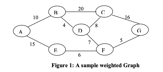
The graph has vertices: A, B, C, D, E, F, G.
Edges with weights:
Edges with weights:
- A-B: 10
- A-E: 15
- B-C: 20
- B-D: 4
- C-D: 8
- C-G: 16
- D-F: 7
- E-F: 6
- F-G: 5
It is connected and undirected.
Kruskal’s Algorithm Demonstration
Kruskal’s algorithm sorts all edges by increasing weight and adds them to the MST if they do not form a cycle (using Union-Find for cycle detection).
- Sort edges by weight:
(B-D: 4), (F-G: 5), (E-F: 6), (D-F: 7), (C-D: 8), (A-B: 10), (A-E: 15), (C-G: 16), (B-C: 20). - Initialize Union-Find: Each vertex is its own component: {A}, {B}, {C}, {D}, {E}, {F}, {G}.
- Add edges one by one:
- Add B-D: 4 (connects {B} and {D} → {B,D}; no cycle). MST: {B-D}, cost = 4.
- Add F-G: 5 (connects {F} and {G} → {F,G}; no cycle). MST: {B-D, F-G}, cost = 9.
- Add E-F: 6 (connects {E} and {F,G} → {E,F,G}; no cycle). MST: {B-D, F-G, E-F}, cost = 15.
- Add D-F: 7 (connects {B,D} and {E,F,G} → {B,D,E,F,G}; no cycle). MST: {B-D, F-G, E-F, D-F}, cost = 22.
- Add C-D: 8 (connects {C} and {B,D,E,F,G} → {B,C,D,E,F,G}; no cycle). MST: {B-D, F-G, E-F, D-F, C-D}, cost = 30.
- Add A-B: 10 (connects {A} and {B,C,D,E,F,G} → {A,B,C,D,E,F,G}; no cycle). MST: {B-D, F-G, E-F, D-F, C-D, A-B}, cost = 40.
- Skip A-E: 15 (A and E already connected; cycle).
- Skip C-G: 16 (C and G already connected; cycle).
- Skip B-C: 20 (B and C already connected; cycle).
- Final MST: Edges {A-B: 10, B-D: 4, C-D: 8, D-F: 7, E-F: 6, F-G: 5}. Total cost: 40.
How to Arrive at the Solution (Kruskal’s)
- Sorting ensures we consider smallest edges first.
- Union-Find efficiently checks cycles (find if roots are same) and merges components (union by rank/path compression for O(α(E)) amortized time, where α is inverse Ackermann).
- Stop after |V|-1 = 6 edges. The greedy choice avoids cycles while minimizing total weight.
Prim’s Algorithm Demonstration
Using the pseudocode above, starting from vertex A (arbitrary choice). We use a priority queue for minimum keys.
- Initialize:
- inMST: All False.
- key: All ∞ except key[A] = 0.
- parent: All -1.
- PQ: All vertices, min is A.
- Iterations:
- Extract A (key=0). inMST[A]=True. Update neighbors: key[B]=10 (parent[B]=A), key[E]=15 (parent[E]=A).
- Extract B (min key=10). inMST[B]=True. Update: key[D]=4 (parent[D]=B), key[C]=20 (parent[C]=B). (Ignore A.)
- Extract D (min key=4). inMST[D]=True. Update: key[C]=8 (better than 20, parent[C]=D), key[F]=7 (parent[F]=D). (Ignore B.)
- Extract F (min key=7). inMST[F]=True. Update: key[E]=6 (better than 15, parent[E]=F), key[G]=5 (parent[G]=F). (Ignore D.)
- Extract G (min key=5). inMST[G]=True. Update: key[C]=8 (no change). (Ignore F.)
- Extract E (min key=6). inMST[E]=True. Update: No better updates. (Ignore A, F.)
- Extract C (min key=8). inMST[C]=True. No better updates. (Ignore B, D, G.)
- Final MST: From parents: B←A (10), D←B (4), F←D (7), G←F (5), E←F (6), C←D (8). Edges {A-B: 10, B-D: 4, D-C: 8, D-F: 7, F-E: 6, F-G: 5}. Total cost: 40.
How to Arrive at the Solution (Prim’s)
- Start from A and grow the tree by always adding the cheapest edge to the fringe (priority queue handles this).
- Updates ensure each vertex's key is the minimum possible at each step.
- Different starting vertex (e.g., G) may yield a different tree but same cost, as the algorithm is correct for connected graphs.
Question:-3(b)
Write the Dijkstra’s shortest path algorithm. Also, find the time complexity of this shortest path algorithm. Find the shortest paths from the vertex ‘A’ using Dijkstra’s shortest path algorithm for the graph given in Figure 1. Show all the steps of computation.
Answer:
Dijkstra’s Shortest Path Algorithm
Dijkstra’s algorithm is a greedy algorithm that finds the shortest paths from a single source vertex to all other vertices in a connected, undirected or directed graph with non-negative edge weights. It maintains a set of vertices whose shortest paths are finalized and grows it by selecting the vertex with the minimum distance estimate.
Pseudocode
Dijkstra(Graph G = (V, E), weights w: E → R ≥ 0, source s ∈ V):
    // Initialize
    dist = array of size |V|, initialized to infinity  // Shortest distance from s
    prev = array of size |V|, initialized to -1  // Previous vertex in path
    dist[s] = 0

    // Priority queue (min-heap) for vertices not yet finalized, keyed by dist
    PQ = priority_queue of all vertices, keyed by dist values

    while PQ is not empty:
        u = extract_min(PQ)  // Vertex with smallest dist

        for each neighbor v of u:
            if dist[v] > dist[u] + w(u, v):
                dist[v] = dist[u] + w(u, v)
                prev[v] = u
                update PQ with new dist for v  // Decrease key operation

    // To reconstruct path to a target t: backtrack from t using prev until s
    return dist, prev
Time Complexity
- With a binary heap for the priority queue and adjacency list representation:
- Extract-min: O(V log V) total (V extractions).
- Decrease-key: O(E log V) total (up to E updates).
- Overall: O((V + E) log V), which simplifies to O(E log V) since E ≥ V-1 in connected graphs.
- For dense graphs (E ≈ V²) using a simple array for minimum selection (no heap): O(V²).
- The O(E log V) variant is common for sparse graphs and assumes a heap that supports efficient decrease-key (e.g., binary or Fibonacci heap; Fibonacci reduces to amortized O(E + V log V)).
Demonstration on the Given Graph: Shortest Paths from A
The graph has vertices A, B, C, D, E, F, G and the edges with weights as shown (undirected, so bidirectional). We apply Dijkstra’s from source A, showing step-by-step updates. We use a priority queue (min-heap) for the next vertex selection.
Initialization
- dist: [A: 0, B: ∞, C: ∞, D: ∞, E: ∞, F: ∞, G: ∞]
- prev: [all -1]
- PQ: All vertices (min keyed on dist; initially A at 0, others ∞)
Step-by-Step Computation
We tabulate the process: each iteration extracts the minimum dist vertex u, then relaxes (updates) its neighbors.
| Iteration | Extracted u (dist[u]) | Updates to Neighbors |
|---|---|---|
| 1 | A (0) | - B: dist[B] = 0 + 10 = 10 (prev[B] = A) - E: dist[E] = 0 + 15 = 15 (prev[E] = A) Current dist: [A:0, B:10, C:∞, D:∞, E:15, F:∞, G:∞] |
| 2 | B (10) | - C: dist[C] = 10 + 20 = 30 (prev[C] = B) - D: dist[D] = 10 + 4 = 14 (prev[D] = B) (A already extracted, ignored) Current dist: [A:0, B:10, C:30, D:14, E:15, F:∞, G:∞] |
| 3 | D (14) | - C: dist[C] = 14 + 8 = 22 (< 30, update; prev[C] = D) - F: dist[F] = 14 + 7 = 21 (prev[F] = D) (B already extracted, ignored) Current dist: [A:0, B:10, C:22, D:14, E:15, F:21, G:∞] |
| 4 | E (15) | - F: 15 + 6 = 21 (== 21, no update) (A already extracted, ignored) Current dist: [A:0, B:10, C:22, D:14, E:15, F:21, G:∞] |
| 5 | F (21) | - G: dist[G] = 21 + 5 = 26 (prev[G] = F) (D, E already extracted, ignored) Current dist: [A:0, B:10, C:22, D:14, E:15, F:21, G:26] |
| 6 | C (22) | - G: 22 + 16 = 38 (> 26, no update) (B, D already extracted, ignored) Current dist: [A:0, B:10, C:22, D:14, E:15, F:21, G:26] |
| 7 | G (26) | (C, F already extracted, ignored) Current dist: [A:0, B:10, C:22, D:14, E:15, F:21, G:26] |
PQ is now empty; all vertices processed.
Final Shortest Distances from A
- A: 0
- B: 10
- C: 22
- D: 14
- E: 15
- F: 21
- G: 26
Shortest Paths from A (Reconstructed using prev)
- To A: A (distance 0)
- To B: A → B (distance 10)
- To C: A → B → D → C (distance 10 + 4 + 8 = 22)
- To D: A → B → D (distance 10 + 4 = 14)
- To E: A → E (distance 15)
- To F: A → B → D → F (distance 10 + 4 + 7 = 21)
Note: Alternative path A → E → F (15 + 6 = 21) has the same distance; the algorithm found one via D. - To G: A → B → D → F → G (distance 10 + 4 + 7 + 5 = 26)
Note: Alternative A → E → F → G (15 + 6 + 5 = 26) equivalent.
How to Arrive at the Solution
- Initialization: Set source distance to 0, others to infinity.
- Relaxation: For each extracted u, check if a shorter path to v exists via u; update if so.
- Priority Queue: Ensures the next u is always the one with the current smallest dist (greedy choice).
- Correctness: Relies on non-negative weights; once a vertex is extracted, its dist is finalized (no shorter path can be found later).
- The steps guarantee optimality by the invariant: at each extraction, dist[u] is the true shortest path.
Question:-3(c)
Explain the algorithm to find the optimal Binary Search Tree. Demonstrate this algorithm to find the Optimal Binary Search Tree for the following probability data (where
Answer:
Algorithm to Find the Optimal Binary Search Tree
The optimal binary search tree (BST) problem involves constructing a BST that minimizes the expected search cost, given probabilities
The expected search cost is defined as
The algorithm uses dynamic programming:
- Let
- Let
- Base cases:
- For empty subtrees (
- For empty subtrees (
- Recurrence:
- To track the tree structure, record
- Compute in order of increasing subtree size
- The optimal cost is
Time Complexity
- The DP fills an
- Total:
Demonstration for the Given Probabilities
Given
We assume the keys are
Step-by-Step Computation
We compute
- Length
- Length
- Length
- r=1:
- r=2:
- r=1:
- r=2:
- r=3:
- r=2:
- r=3:
- r=4:
- r=3:
- Length
- r=1:
- r=2:
- r=3:
- r=1:
- r=2:
- r=3:
- r=4:
- r=2:
- Length
- r=1:
- r=2:
- r=3:
- r=4:
- r=1:
How to Arrive at the Solution
- DP Table Construction: Start with empty subtrees (cost 0). For each larger subtree, compute the probability mass
- Optimal Cost:
- Tree Construction: Use the root table recursively:
- Root:
- Left subtree (keys 1-2): Root
- Left of
- Right of
- Left of
- Right subtree (keys 4-4): Root
- Root:
The optimal BST is:
- Root:
- Left:
- Left:
- Right: None
- Left:
- Right:
- Left:
This structure favors higher-probability keys (
Question:-3(d)
Given the following sequence of chain multiplication of the matrices. Find the optimal way of multiplying these matrices:
Answer:
Algorithm to Find the Optimal Matrix Chain Multiplication
The matrix chain multiplication problem involves finding the most efficient way to multiply a sequence of matrices
This is solved using dynamic programming:
- Let
- Let
- Dimensions are given as
- Recurrence:
- Compute for increasing chain lengths
- The optimal cost is
Time Complexity
- The DP table is
- Total:
Demonstration for the Given Matrices
Given matrices:
Dimensions array
Step-by-Step Computation
We compute
- Length
- Length
- Length
- Length
Optimal Parenthesization
- Reconstruct using
- Left:
- Right:
- Final multiplication:
How to Arrive at the Solution
- DP Approach: Build costs bottom-up, considering all possible splits. The cost includes previous subproblems plus the multiplication cost.
- Optimality: The recurrence ensures the minimum by trying all
- The chosen split minimizes the total scalar multiplications, validated by the computed
Question:-3(e)
Explain the Rabin Karp algorithm for string matching with the help of an example. Find the time complexity of this algorithm.
Answer:
Rabin-Karp Algorithm for String Matching
The Rabin-Karp algorithm is a string-searching algorithm that uses hashing to efficiently find occurrences of a pattern (substring) within a larger text. It avoids comparing every possible substring character-by-character by instead computing hash values for the pattern and sliding windows of the text. If the hash of a text window matches the pattern's hash, a full character comparison is performed to confirm a match (to handle potential hash collisions).
Key Concepts
- Hashing: Treat strings as numbers in a large base (e.g., base
- Rolling Hash: Efficiently update the hash for the next window in constant time, rather than recomputing from scratch. This is done by subtracting the contribution of the outgoing character and adding the incoming one.
- Modulo Operation: Use a large prime modulus
- Handling Collisions: Hashes may collide (different strings with same hash), so always verify matches with direct comparison.
Steps of the Algorithm
- Let
- Choose a base
- Precompute
- Compute the hash of the pattern:
- Compute the initial hash of the first
- If
- For each subsequent window
- Update
(Handle negative values by adding - If
- Update
Example
Consider the text
- Precompute
- Pattern hash (
7227 ÷ 13 = 555*13=7215, remainder 12. So - Initial text window "ABC":
Hashes match (12==12). Compare strings: "ABC" == "ABC" → Match at index 0. - Next window (i=1): "BCD"
Update:
First, 659=585 mod 13: 585-4513=585-585=0, so 12 - 0 =12.
1012=120 +68=188 mod13: 188-1413=188-182=6.
"BCD" hash=6 ≠12 → No match. - Next (i=2): "CDA"
Update from previous: Subtract C's contrib (679 mod13:679=603,603-46*13=603-598=5), so 6-5=1, then 10=10 +65=75 mod13=75-513=75-65=10 ≠12. - Next (i=3): "DAB" → Continues, no match.
- Next (i=4): "ABC" → Hash will compute to 12, match at index 4 (after update steps).
- And so on. Matches found at 0 and 4.
In a real implementation, characters are treated as integers, and larger primes reduce collisions.
Time Complexity
- Preprocessing: O(m) to compute pattern hash and initial text hash.
- Sliding Window: O(n - m + 1) updates, each O(1) time.
- Verifications: In the average case, few collisions, so O(m) per true match, leading to overall average O(n + m).
- Worst Case: If every hash matches (many collisions), verify all n-m+1 windows, each O(m), so O((n - m + 1) * m) ≈ O(nm). With a good hash (large prime), collisions are rare, making average close to O(n + m).
Question:-4(a)
Explain the term Decision problem with the help of an example. Define the following problems and identify if they are decision problem or optimisation problem? Give reasons in support of your answer.
(i) Travelling Salesman Problem
(ii) Graph Colouring Problem
(iii) 0-1 Knapsack Problem
(ii) Graph Colouring Problem
(iii) 0-1 Knapsack Problem
Answer:
❓ Decision Problem
A decision problem is a question with a yes/no answer.
Example:
"Is there a path from node A to node B in a graph with length ≤ k?"
Example:
"Is there a path from node A to node B in a graph with length ≤ k?"
🧳 (i) Travelling Salesman Problem (TSP)
- Standard form: Find the shortest route visiting each city exactly once and returning to the start.
- This is an optimization problem (minimize route length).
- Decision version: "Is there a route of length ≤ k?"
- This is a decision problem.
Reason: The core question seeks a minimum value, but it can be framed as a decision problem by asking if a solution exists within a bound.
🎨 (ii) Graph Colouring Problem
- Standard form: Assign colours to vertices so no adjacent vertices share a colour, using the fewest colours.
- This is an optimization problem (minimize colours).
- Decision version: "Can the graph be coloured with k colours?"
- This is a decision problem.
Reason: The goal is to minimize colours, but it is often treated as a decision problem for complexity analysis (e.g., k-colouring).
🎒 (iii) 0-1 Knapsack Problem
- Standard form: Select items to maximize profit without exceeding weight capacity.
- This is an optimization problem (maximize profit).
- Decision version: "Is there a subset of items with profit ≥ P and weight ≤ W?"
- This is a decision problem.
Reason: The natural form seeks maximum profit, but it can be converted to a decision problem by introducing a profit threshold.
✅ Summary:
- All three are optimization problems in their standard form.
- Each has a decision version used in computational complexity theory (e.g., NP-completeness).
- Decision problems are easier to analyze in terms of complexity classes.
Question:-4(b)
What are P and NP class of Problems? Explain each class with the help of at least two examples.
Answer:
🧠 P and NP Classes of Problems
🟢 Class P (Polynomial Time)
Definition: Problems that can be solved by a deterministic Turing machine in polynomial time (
Examples:
- Sorting a list
- Algorithms like Merge Sort run in
- Algorithms like Merge Sort run in
- Finding the shortest path in a graph (Dijkstra's algorithm)
- Runs in
- Runs in
🔴 Class NP (Nondeterministic Polynomial Time)
Definition: Problems whose solutions can be verified in polynomial time by a deterministic Turing machine. Note: NP does NOT mean "not polynomial"; it means "nondeterministic polynomial".
Examples:
- Boolean Satisfiability (SAT)
- Given a Boolean formula, is there an assignment of variables that makes it true?
- Verification: Check if a given assignment satisfies the formula in linear time.
- Traveling Salesman Problem (Decision Version)
- Is there a route of length ≤ k?
- Verification: Check if a given route visits all cities and has length ≤ k in polynomial time.
🔑 Key Points:
- P ⊆ NP (If you can solve it, you can verify it).
- Open Question: Is P = NP? (One of the Millennium Prize Problems).
- NP includes problems that are "easy" to verify but may be "hard" to solve.
📊 Comparison:
| Class | Solvable in Poly-Time | Verifiable in Poly-Time | Examples |
|---|---|---|---|
| P | Yes | Yes | Sorting, Shortest Path |
| NP | Unknown | Yes | SAT, TSP |
Understanding P and NP is crucial for complexity theory and cryptography! 🎯
Question:-4(c)
Define the NP-Hard and NP-Complete problem. How are they different from each other. Explain the use of polynomial time reduction with the help of an example.
Answer:
🧩 NP-Hard and NP-Complete Problems
🔴 NP-Hard
A problem is NP-hard if it is at least as hard as the hardest problems in NP. This means any problem in NP can be reduced to it in polynomial time. NP-hard problems may not be in NP themselves.
Example:
- Halting Problem (undecidable, but NP-hard)
- Traveling Salesman Problem (optimization version)
🟠 NP-Complete
A problem is NP-complete if it is:
- In NP (verifiable in polynomial time).
- NP-hard (all NP problems reduce to it).
Examples:
- Boolean Satisfiability (SAT)
- Graph Coloring
- Subset Sum
🔍 Key Differences:
| NP-Hard | NP-Complete |
|---|---|
| May not be in NP | Must be in NP |
| Includes optimization problems | Typically decision problems |
| e.g., Halting Problem | e.g., 3-SAT |
⏱️ Polynomial-Time Reduction
A reduction transforms problem A to problem B in polynomial time such that solving B solves A. Used to prove NP-hardness.
Example: Reducing 3-SAT to Graph Coloring:
- Show that if we can solve Graph Coloring quickly, we can solve 3-SAT quickly.
- Construct a graph from a 3-CNF formula where coloring the graph with k colors implies a satisfying assignment.
This proves Graph Coloring is NP-hard if 3-SAT is NP-hard.
Question:-4(d)
Define the following Problems:
(i) SAT Problem
(ii) Clique Problem
(iii) Hamiltonian Cycle Problem
(iv) Subset Sum Problem
(ii) Clique Problem
(iii) Hamiltonian Cycle Problem
(iv) Subset Sum Problem
Answer:
📌 (i) SAT Problem (Boolean Satisfiability Problem)
Definition: Given a Boolean formula (e.g., in conjunctive normal form), is there an assignment of truth values to variables that makes the entire formula true?
Example:
Formula:
Is there values for
Formula:
Is there values for
👥 (ii) Clique Problem
Definition: A clique is a complete subgraph (every pair of vertices connected). The decision problem: Does a graph contain a clique of size
Example:
In a social network, is there a group of
In a social network, is there a group of
🔁 (iii) Hamiltonian Cycle Problem
Definition: Does a graph contain a cycle that visits every vertex exactly once and returns to the start?
Example:
Can a salesperson visit each city exactly once and return home?
Can a salesperson visit each city exactly once and return home?
💰 (iv) Subset Sum Problem
Definition: Given a set of integers and a target sum
Example:
Set:
Set: